C-7.27.2 effective length method
PDF page 716 · AISC 360-22
The effective length method (though it was not originally identified by this name) has been used in various forms in the AISC Specification since 1961. The provisions are essentially the same as those in Appendix 7 of the 2010 AISC Specification (AISC, 2010).
These provisions, together with the use of a column effective length greater than the actual length for calculating available strength in some cases, account for the effects of initial out-of-plumbness and member stiffness reductions due to the spread of plasticity. No stiffness reduction is required in the analysis.
The effective length, , for column buckling based upon elastic or inelastic stability theory, or alternatively the equivalent elastic column buckling stress, , is used to calculate an axial compressive strength, , through an empirical column curve that accounts for geometric imperfections and distributed yielding including the effects of residual stresses. This column strength is then combined with the available flexural strength, , and second-order member forces, and , in the beam-column interaction equations.
Braced Frames. Braced frames are commonly idealized as vertically cantilevered pin-connected truss systems, ignoring any secondary moments within the system. The effective length factor, , of components of the braced frame is normally taken
as 1.0, unless a smaller value is justified by structural analysis and the member and connection design is consistent with this assumption. If connection fixity is modeled in the analysis, the resulting member and connection moments must be accommodated in the design.
If is used for the calculation of the nominal compressive strength, , in braced frames, the additional demands on the stability bracing systems and the influence on the second-order moments in beams providing restraint to the columns must be considered. The provisions in Appendix 6 do not address the additional demands on bracing members from the use of . Generally, a and second-order elastic analysis is necessary for calculation of the second-order moments in beams providing restraint to column members designed based on ; therefore, design using is recommended, except in those special situations where the additional calculations are deemed justified.
The effective length, , may be taken as for both in-plane and out-of-plane buckling of concentrically loaded compression braces in X-braced frames, where is the overall length of the brace between work points, with identically sized brace members when the compression and tension braces are attached at the midpoint and the magnitude of compression and tension forces in the braces are approximately equal (McGuire et al., 2000). Greater unbraced lengths for out-of-plane buckling may be required for X-braced frames with unbalanced brace forces, particularly those with discontinuous midpoint connections (Davaran, 2001). Shorter unbraced lengths may also be justified (El-Tayem and Goel, 1986; Picard and Beaulieu, 1987; Nair, 1997; Moon et al., 2008).
Moment Frames. Moment frames rely primarily upon the flexural stiffness of the connected beams and columns for stability. Stiffness reductions due to shear deformations may require consideration when bay sizes are small and/or members are deep.
When the effective length method is used, the design of all beam-columns in moment frames must be based on an effective length, , greater than the actual laterally unbraced length, , except when specific exceptions based upon high structural stiffness are met. When the sidesway amplification, or , is equal to or less than 1.1 , the frame design may be based on the use of for the columns. This simplification for stiffer structures results in a maximum error in the in-plane beam-column strength checks of Chapter H (White and Hajjar, 1997a). When the sidesway amplification is larger, must be calculated.
A wide range of methods has been suggested in the literature for the calculation of -factors (Kavanagh, 1962; Johnston, 1976; LeMessurier, 1977; ASCE, 1997; White and Hajjar, 1997b). These range from simple idealizations of single columns, as shown in Table C-A-7.1, to complex buckling solutions for specific frames and loading conditions. In some types of frames, -factors are easily estimated or calculated and are a convenient tool for stability design. In other types of structures, accurate -factors are determined by tedious hand procedures, and system stability may be assessed more effectively with the direct analysis method.
TABLE C-A-7.1
Approximate Values of Effective Length Factor, K
| Buckled shape of column is shown by dashed line | (a) | (b) | (c) | (d) | (e) | (f) |
|---|---|---|---|---|---|---|
| mm | mm | mm | mm | mm | mm | |
| Theoretical K value | 0.5 | 0.7 | 1.0 | 1.0 | 2.0 | 2.0 |
| Recommended design value when ideal conditions are approximated | 0.65 | 0.8 | 1.0 | 1.2 | 2.1 | 2.0 |
| End condition code | [Icon 1] | Rotation fixed and translation fixed | ||||
| [Icon 2] | Rotation free and translation fixed | |||||
| [x] | Rotation fixed and translation free | |||||
| १ | Rotation free and translation free | |||||
| [Icon 5] | Rotation fixed, horizontal translation fixed, and vertical translation free | |||||
| [Icon 6] | Rotation free, horizontal translation fixed, and vertical translation free | |||||
Alignment Charts. The most common method for determining is through use of the alignment charts, which are shown in Figure C-A-7.1 for frames with sidesway inhibited and Figure C-A-7.2 for frames with sidesway uninhibited (Kavanagh, 1962). These charts are based on assumptions of idealized conditions, which seldom exist in real structures, as follows:
-
(a) Behavior is purely elastic.
-
(b) All members have a constant cross section.
-
(c) All joints are rigid.
-
(d) For columns in frames with sidesway inhibited, rotations at opposite ends of the restraining beams are equal in magnitude and opposite in direction, producing single curvature bending.
-
(e) For columns in frames with sidesway uninhibited, rotations at opposite ends of the restraining beams are equal in magnitude and direction, producing reverse curvature bending.
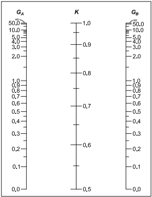
Figure description:
Effective Length Factor (K Nomogram Sidesway Inhibited
Nomogram Scales
Annotations
- G_A (text_label - position: Top of left scale)
- K (text_label - position: Top of center scale)
- G_B (text_label - position: Top of right scale)
| Scale G_A Labeled Values | Scale K Labeled Values | Scale G_B Labeled Values |
|---|---|---|
| ∞ | 1.0 | ∞ |
| 50.0 | 0.9 | 50.0 |
| 10.0 | 0.8 | 10.0 |
| 5.0 | 0.7 | 5.0 |
| 4.0 | 0.6 | 4.0 |
| 3.0 | 0.5 | 3.0 |
| 2.0 | 2.0 | |
| 1.0 | 1.0 | |
| 0.9 | 0.9 | |
| 0.8 | 0.8 | |
| 0.7 | 0.7 | |
| 0.6 | 0.6 | |
| 0.5 | 0.5 | |
| 0.4 | 0.4 | |
| 0.3 | 0.3 | |
| 0.2 | 0.2 | |
| 0.1 | 0.1 | |
| 0.0 | 0.0 |
Notes: This figure is an alignment chart (nomogram used in structural engineering to determine the effective length factor (K for columns in frames where sidesway is inhibited. It consists of three vertical scales. The outer scales G_A and G_B (representing stiffness ratios at column ends are identical, non-linear, and range from 0.0 to infinity. The central scale for K is linear and ranges from 0.5 to 1.0. To use the chart, a straight line is drawn between known values on the G_A and G_B scales; the intersection with the K scale provides the effective length factor.)))
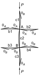
Figure description:
Key Information:
- Subject: Structural diagram of a braced frame segment for alignment chart derivation (sidesway inhibited.
- Load: Vertical axial compressive force applied to the column stack.
- Nodes: Two primary interior joints labeled A and B.
- Columns: Vertical members identified as c1 (top, c2 (middle/target, and c3 (bottom.)))
- Beams: Horizontal members identified as b1, b2 (connected at Node A and b3, b4 (connected at Node B.))
- Deformation: Curvature is shown for all members based on joint rotations and , representing the buckling mode of a continuous frame where lateral translation is prevented.
Fig. C-A-7.1. Alignment chart—sidesway inhibited (braced frame).
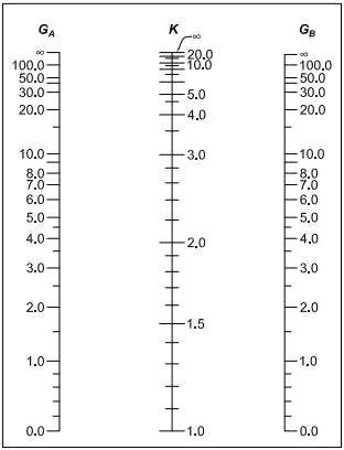
Figure description:
Nomogram for GA, K, and GB Effective Length Factor for Columns in Unbraced Frames
Nomogram Scales for GA, K, and GB
| GA | K | GB |
|---|---|---|
| 0.0 | 1.0 | 0.0 |
| 1.0 | 1.5 | 1.0 |
| 2.0 | 2.0 | 2.0 |
| 3.0 | 3.0 | 3.0 |
| 4.0 | 4.0 | 4.0 |
| 5.0 | 5.0 | 5.0 |
| 6.0 | 10.0 | 6.0 |
| 7.0 | 20.0 | 7.0 |
| 8.0 | ∞ | 8.0 |
| 10.0 | "" | 10.0 |
| 20.0 | "" | 20.0 |
| 30.0 | "" | 30.0 |
| 50.0 | "" | 50.0 |
| 100.0 | "" | 100.0 |
| ∞ | "" | ∞ |
Notes: This figure is an alignment chart (nomogram used in structural engineering to determine the effective length factor (K for columns in frames. The GA and GB scales are identical log-like scales ranging from 0.0 to infinity. The K scale is a central scale ranging from 1.0 to infinity. The table lists the primary labeled values found on each scale.))
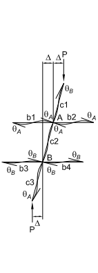
Figure description:
Structural Model: Diagram of a subframe for a moment-resisting frame with uninhibited sidesway.
Key Entities:
- Joints: Node A (top center and Node B (bottom center.
- Columns: Vertical members labeled c1, c2, and c3; c2 connects Node A and Node B.
- Beams: Horizontal members b1 and b2 connected to Node A; b3 and b4 connected to Node B.
Key Parameters:
- Load (P: Axial vertical force applied to the column line.
- Displacement (: Lateral sidesway translation of the joints.
- Rotations: Joint rotations denoted as at Node A and at Node B.
- Purpose: Illustrates the deformation used to derive alignment charts for calculating the effective length factor (K in unbraced frames.
Fig. C-A-7.2. Alignment chart—sidesway uninhibited (moment frame).
- (f) The stiffness parameter of all columns is equal.
- (g) Joint restraint is distributed to the column above and below the joint in proportion to for the two columns.
- (h) All columns buckle simultaneously.
- (i) No significant axial compression force exists in the girders.
- (j) Shear deformations are neglected.
The alignment chart for sidesway inhibited frames shown in Figure C-A-7.1 is based on the following equation:
The alignment chart for sidesway uninhibited frames shown in Figure C-A-7.2 is based on the following equation:
(C-A-7-2)
where
(C-A-7-3)
The subscripts and refer to the joints at the ends of the column being considered. The symbol indicates a summation of all members rigidly connected to that joint and located in the plane in which buckling of the column is being considered. is the modulus of elasticity of the column, is the moment of inertia of the column, and is the unsupported length of the column. is the modulus of elasticity of the girder, is the moment of inertia of the girder, and is the unsupported length of the girder or other restraining member. and are taken about axes perpendicular to the plane of buckling being considered. The alignment charts are valid for different materials if an appropriate effective rigidity, , is used in the calculation of .
It is important to remember that the alignment charts are based on the assumptions of idealized conditions previously discussed—and that these conditions seldom exist in real structures. Therefore, adjustments are often required.
Adjustments for Columns with Differing End Conditions. For column ends supported by, but not rigidly connected to, a footing or foundation, is theoretically infinity but, unless designed as a true friction-free pin, may be taken as 10 for practical designs. If the column end is rigidly attached to a properly designed footing, may be taken as 1.0. Smaller values may be used if justified by analysis.
Adjustments for Girders with Differing End Conditions. For sidesway inhibited frames, these adjustments for different girder end conditions may be made:
- (a) If rotation at the far end of a girder is prevented, multiply of the member by 2.
- (b) If the far end of the girder is pinned, multiply of the member by 1.5 .
For sidesway uninhibited frames and girders with different boundary conditions, the modified girder length, , should be used in place of the actual girder length,
where
(C-A-7-4)
is the far end girder moment and is the near end girder moment from a firstorder lateral analysis of the frame. The ratio of the two moments is positive if the girder is in reverse curvature. If is more than 2.0 , then becomes negative, in which case is negative and the alignment chart equation must be used. For sidesway uninhibited frames, the following adjustments for different girder end conditions may be made:
- (a) If rotation at the far end of a girder is prevented, multiply of the member by .
(b) If the far end of the girder is pinned, multiply of the member by .
Adjustments for Girders with Significant Axial Load. For both sidesway conditions, multiply by the factor , where is the axial load in the girder and is the in-plane buckling load of the girder based on .
Adjustments for Column Inelasticity. For both sidesway conditions, replace with for all columns in the expression for and . It is noted that , as defined in Section C2.3, is being used as a simple conservative approximation for the expression that appeared in previous editions of the Commentary (AISC, 2005b). Adjustments for column inelasticity may be conservatively ignored and will result in larger -factors.
Adjustments for Connection Flexibility. One important assumption in the development of the alignment charts is that all beam-column connections are fully restrained (FR) connections. When the far end of a beam does not have an FR connection that behaves as assumed, an adjustment must be made. When a beam connection at the column under consideration is a shear-only connection, that is, there is no moment, then that beam cannot participate in the restraint of the column, and it cannot be considered in the term of the equation for . Only FR connections can be used directly in the determination of . Partially restrained (PR) connections with a documented moment-rotation response can be utilized, but of each beam must be adjusted to account for the connection flexibility. ASCE (1997) provides a detailed discussion of frame stability with PR connections.
Combined Systems. When combined systems are used, all the systems must be included in the structural analysis. Consideration must be given to the variation in stiffness inherent in concrete or masonry shear walls due to various degrees to which these elements may experience cracking. This applies to load combinations for serviceability as well as strength. It is prudent for the designer to consider a range of possible stiffnesses, as well as the effects of shrinkage, creep, and load history, in order to envelope the likely behavior and provide sufficient strength in all interconnecting elements between systems. Following the analysis, the available strength of compression members in moment frames must be assessed with effective lengths calculated as required for moment-frame systems; other compression members may be assessed using .
Gravity-Only Columns and Distribution of Sidesway Instability Effects. Columns in gravity framing systems can be designed as pin-ended columns with . However, the destabilizing effects ( effects) of the gravity loads on all such columns, and the load transfer from these columns to the lateral force-resisting system, must be accounted for in the design of the lateral force-resisting system.
It is important to recognize that sidesway instability of a building is a story phenomenon involving the sum of the sway resistances of all the lateral force-resisting elements in the story and the sum of the factored gravity loads in the columns in that story. No individual column in a story can buckle in a sidesway mode without the entire story buckling.
If every column in a story is part of a moment frame and each column is designed to support its own axial load, , and moment such that the contribution of each column to the lateral stiffness or to the story buckling load is proportional to the axial load supported by the column, all the columns will buckle simultaneously. Under this idealized condition, there is no interaction among the columns in the story; column sway instability and frame instability occur at the same time. Typical framing, however, does not meet this idealized condition, and real systems redistribute the story effects to the lateral force-resisting elements in that story in proportion to their stiffnesses. This redistribution can be accomplished using such elements as floor diaphragms or horizontal trusses.
In a building that contains columns that contribute little or nothing to the sway stiffness of the story, such columns are referred to as leaning or gravity-only columns. These columns can be designed using , but the lateral force-resisting elements in the story must be designed to support the destabilizing effects developed from the loads on these gravity-only columns. The redistribution of effects among columns must be considered in the determination of and for all the columns in the story for the design of moment frames. The proper -factor for calculation of in moment frames, accounting for these effects, is denoted in the following by the symbol .
Effective Length for Story Stability. Two approaches for evaluating story stability are recognized: the story stiffness approach (LeMessurier, 1976, 1977) and the story buckling approach (Yura, 1971). Additionally, a simplified approach proposed by LeMessurier (1995) is also discussed.
The column effective length factor associated with lateral story buckling is expressed as in the following discussions. The value of determined from Equation C-A-7-5 or Equation C-A-7-8 may be used directly in the equations of Chapter E. However, it is important to note that this substitution is not appropriate when calculating the story buckling mode as the summation of . Also, note that the value of calculated using by either method cannot be taken to be greater than the value of determined based on sidesway-inhibited buckling.
Story Stiffness Approach. For the story stiffness approach, is defined as
(C-A-7-5)
Specification for Structural Steel Buildings, August 1, 2022 AMERICAN INSTITUTE OF STEEL CONSTRUCTION
in which is used to approximate the influence of effects on the sidesway stiffness of the columns in a story and is defined in Equation A-8-8 as
(C-A-7-6)
where , and are as defined in Appendix 8, Section 8.1.3.
It is possible that certain columns, having only a small contribution to the lateral force resistance in the overall frame, will have a value less than 1.0 based on the term to the left of the inequality. The limit on the right-hand side is a minimum value for that accounts for the interaction between sidesway and non-sidesway buckling (ASCE, 1997; White and Hajjar, 1997b). The term is the shear in the column under consideration, produced by the lateral forces used to compute .
Equation C-A-7-5 can be reformulated to obtain the column buckling load, , as
(C-A-7-7)
in Equations C-A-7-5 to C-A-7-7 includes all columns in the story, including any gravity-only columns, and is for the column under consideration. The column buckling load, , calculated from Equation C-A-7-7, may be larger than but may not be larger than the limit on the right-hand side of this equation.
In Appendix 8, the story stiffness approach is the basis for the calculation for effects. In Equation A-8-7, the buckling load for the story is expressed in terms of the story drift ratio, , from a first-order lateral load analysis at a given applied lateral load level. In preliminary design, may be taken in terms of a target maximum value for this drift ratio. This approach focuses the engineer's attention on the most fundamental stability requirement in building frames: providing adequate overall story stiffness in relation to the total vertical load, , supported by the story. The elastic story stiffness expressed in terms of the drift ratio and the total horizontal load acting on the story is .
Story Buckling Approach. For the story buckling approach, is defined as
(C-A-7-8)
where is defined as the value of determined directly from the alignment chart in Figure C-A-7.2.
The value of calculated from Equation C-A-7-8 may be less than 1.0. The limit on the right-hand side is a minimum value for that accounts for the interaction between sidesway and non-sidesway buckling (ASCE, 1997; White and Hajjar, 1997b; Geschwindner, 2002; AISC-SSRC, 2003b). Other approaches to calculating are given in previous editions of this Commentary and the foregoing references.
Equation C-A-7-8 can be reformulated to obtain the column buckling load, , as
(C-A-7-9)
in Equations C-A-7-8 and C-A-7-9 includes all columns in the story, including any gravity-only columns, and is for the column under consideration. The column buckling load, , calculated from Equation C-A-7-9, may be larger than but may not be larger than the limit on the right-hand side of this equation.
LeMessurier Approach. Another simple approach for the determination of (LeMessurier, 1995), based only on the column end moments, is
(C-A-7-10)
In this equation, and are the smaller and larger end moments, respectively, in the column. These moments are determined from a first-order analysis of the frame under lateral load. Column inelasticity is considered in the derivation of this equation. The unconservative error in , when it is based on determined from Equation C-A-7-10, is less than if the following inequality is satisfied:
(C-A-7-11)
where is the sum of the axial yield strengths of all columns in the story that are part of moment frames, if any, in the direction of translation being considered.
Some Conclusions Regarding . Column design using -factors can be tedious and confusing for complex building structures containing gravity-only columns or combined framing systems, particularly where column inelasticity is considered. This confusion can be avoided if the direct analysis method of Chapter C is used, where is always based on . Subject to certain limitations, the direct analysis method may be simplified to the first-order analysis method of Section 7.3. Furthermore, when or is sufficiently low, may be assumed in the effective length method as specified in Section 7.2.3(b).
Comparison of the Effective Length Method and the Direct Analysis Method. Figure C-C2.5(a) shows a plot of the in-plane interaction equation for the effective length method, where the anchor point on the vertical axis, , is determined using an effective length of . Also shown in this plot is the same interaction equation with the first term based on the yield load, . For W-shapes, this in-plane beam-column interaction equation is a reasonable estimate of the internal force state associated with full cross-section plastification.
The versus response of a typical member, obtained from second-order spreadof-plasticity analysis and labeled "actual response," indicates the maximum axial force, , that the member can sustain prior to the onset of instability. The loaddeflection response from a second-order elastic analysis using the nominal geometry and elastic stiffness, as conducted with the effective length method, is also shown.
The “actual response” curve has larger moments than the second-order elastic curve due to the combined effects of distributed yielding and geometric imperfections, which are not included in the second-order elastic analysis.
In the effective length method, the intersection of the second-order elastic analysis curve with the interaction curve determines the member strength. The plot in Figure C-C2.5(a) shows that the effective length method is calibrated to give a resultant axial strength, , consistent with the actual response. For slender columns, the calculation of the effective length, , and is critical to achieving an accurate solution when using the effective length method.
One consequence of the procedure is that it underestimates the actual internal moments under the factored loads, as shown in Figure C-C2.5(a). This is inconsequential for the beam-column in-plane strength check because reduces the effective strength in the correct proportion. However, the reduced moment can affect the design of the beams and connections, which provide rotational restraint to the column. This is of greatest concern when the calculated moments are small and axial loads are large, such that moments induced by column out-of-plumbness can be significant.
The important difference between the direct analysis method and the effective length method is that where the former uses reduced stiffness in the analysis and in the beam-column strength check, the latter uses nominal stiffness in the analysis and from a sidesway buckling analysis in the beam-column strength check. The direct analysis method can be more sensitive to the accuracy of the second-order elastic analysis because analysis at reduced stiffness increases the magnitude of second-order effects. However, this difference is important only at high sidesway amplification levels; at those levels, the accuracy of the calculation of for the effective length method also becomes important.