C-4.24.2 structural design for fire conditions by analysis
PDF page 668 · AISC 360-22
4.2.1 Design-Basis Fire
Once a fuel load has been agreed upon for the occupancy, the designer should demonstrate the effect of various fires on the structure by assessing the temperature-time relationships for various ventilation factors. NFPA 557 (NFPA, 2020b) and SFPE S.01 (SFPE, 2011), as well as other published standards, can be consulted in this regard. These heating effects may result in different structural responses, and it is useful to demonstrate the capability of the structure to withstand such exposures. The effects of a localized fire should also be assessed to ascertain that local damage is not excessive. Based on these results, members, connections, and edge details can be specified to provide a structure that is sufficiently robust.
4.2.1a Localized Fire
Localized fires may occur in large open spaces, such as the pedestrian area of covered malls, concourses of airport terminals, warehouses, and factories, where fuel packages are separated by large aisles or open spaces. In such cases, the radiant heat flux can be estimated by a point source approximation, requiring the heat release rate of the fire and separation distance between the center of the fuel package and the closest surface of the steelwork. The heat release rate can be determined from experimental results or may be estimated if the mass loss rate per unit floor area occupied by the fuel is known; otherwise, a steady-state fire may be assumed.
4.2.1b Post-Flashover Compartment Fires
Caution should be exercised when determining temperature-time profiles for spaces with high aspect ratios, for example, 5:1 or greater, or for large spaces, for example, those with an open (or exposed) floor area in excess of 5,000 ft² (460 m²). In such cases, it is unlikely that all combustibles will burn in the space simultaneously. Instead, burning will be most intense in, or perhaps limited to, the combustibles
nearest to a ventilation source. For modest-sized compartments with low aspect ratios, the temperature history of the design fire can be determined by algebraic equations or computer models, such as those described in the SFPE Handbook of Fire Protection Engineering (SFPE, 2002) or Eurocode Model Code on Fire Engineering (ECCS, 2001).
Caution should be exercised when determining the fire duration for spaces with high aspect ratios, for example, 5:1 or greater, or for large spaces, for example, those with a floor area in excess of 5,000 ft² (460 m²). The principal difficulty lies in obtaining a realistic estimate for the mass loss rate, given that all combustibles within the space may not be burning simultaneously. Failure to recognize uneven burning will result in an overestimation of the mass burning rate and an underestimation of the fire duration by a significant margin. Note: Some computation methods may implicitly determine the duration of the fire, in which case, the calculation of mass loss rate is unnecessary.
Where a parametric curve is used to define a post-flashover fire, the duration is determined by means of the fuel versus ventilation provisions, not explicitly by loss of mass. This clause should not limit the use of temperature-time relationships to those where duration is calculated, as stated in the foregoing, as these tend to be localized fires and external fire.
4.2.1c Exterior Fires
A design guide is available for determining the exposure resulting from an exterior fire (AISI, 1979).
4.2.1d Active Fire-Protection Systems
Due consideration should be given to the reliability and effectiveness of active fire-protection systems when describing the design-basis fire. When an automatic sprinkler system is installed, the total fuel load may be reduced by up to 60% based on Eurocode 1 (CEN, 1991). The maximum reduction in the fuel load should be considered only when the automatic sprinkler system is considered to be of the highest reliability; for example, reliable and adequate water supply, supervision of control valves, regular schedule for maintenance of the automatic sprinkler system developed in accordance with NFPA (2020a), or alterations of the automatic sprinkler system are considered any time alterations for the space are considered.
For spaces with automatic smoke and heat vents, computer models are available to determine the smoke temperature (SFPE, 2002). Reduction in the temperature profile because of smoke and heat vents should only be considered for reliable installations of smoke and heat vents. Therefore, a regular maintenance schedule for the vents needs to be established in accordance with NFPA (2021a).
4.2.2 Temperatures in Structural Systems Under Fire Conditions
The heat transfer analysis may range from lumped analyses, where the structural member is assumed to be at uniform temperature, to three-dimensional analyses. The uniform temperature assumption is appropriate in a “lumped heat capacity analysis”
where a steel column, beam, or truss element is uniformly heated along the entire length and around the entire perimeter of the exposed section and the protection system is uniform along the entire length and around the entire perimeter of the section. In cases with nonuniform heating or where different protection methods are used on different sides of the column, a two-dimensional analysis should be conducted for steel column assemblies. Two-dimensional analyses are also appropriate for beams, bar joists, or truss elements supporting floor or roof slabs. In the case of composite plate shear walls with uniform heating along the width, a one-dimensional analysis can be conducted per unit width of the wall. A two-dimensional or threedimensional analysis may be required for composite plate shear wall systems with nonuniform heating or with special configurations or boundary conditions.
Heat transfer analyses should consider changes in material properties with increasing temperature for all materials included in the assembly. This may be done in the lumped heat capacity analysis using an effective property value, determined at a temperature near the estimated midpoint of the temperature range expected to be experienced by that component over the duration of the exposure. In the one-, two-, and three-dimensional analyses, the variation in properties with temperature should be explicitly included.
The boundary conditions for the heat transfer analysis should consider radiation heat transfer in all cases and convection heat transfer if the exposed element is submerged in the smoke or is being subjected to flame impingement. The presence of fire-resistive materials in the form of insulation, heat screens, or other protective measures should be taken into account, if appropriate.
Lumped Heat Capacity Analysis. This first-order analysis to predict the temperature rise of steel structural members can be conducted using algebraic equations iteratively. This approach assumes that the steel member has a uniform temperature, applicable to cases where the steel member is unprotected or uniformly protected on all sides, and is exposed to fire around the entire perimeter of the assembly containing the steel member. Caution should be used when applying this method to steel beams supporting floor and roof slabs, as the approach will overestimate the temperature rise in the beam. In addition, where this analysis is used as input for the structural analysis of a fire-exposed steel beam supporting a floor and roof slab, the thermally induced moments will not be simulated as a result of the uniform temperature assumption.
The fire temperature needs to be determined based on the results of the design fire analysis. As alternatives, the standard time-temperature curves indicated in ASTM E119 (ASTM, 2020d) for building fires or ASTM E1529 (ASTM, 2016) for petrochemical fires may be selected.
Unprotected Steel Members. The temperature rise in an unprotected steel section in a short time period is determined by
(C-A-4-2)
TABLE C-A-4.2
Guidelines for Estimating εF
| Type of Assembly | εF |
|---|---|
| Member exposed on all sides | 0.7 |
| Floor beam: Embedded in concrete floor slab, with only bottom flange of beam exposed to fire | 0.5 |
| Floor beam, with concrete slab resting on top flange of beam | |
| • Flange width-to-beam depth ratio ≥ 0.5 | 0.5 |
| • Flange width-to-beam depth ratio < 0.5 | 0.7 |
where
where = heat perimeter, in. (mm) = temperature of the fire, °F (°C) = temperature of the steel, °F (°C) = weight (mass) per unit length, lb/ft (kg/m) = heat transfer coefficient, Btu/(ft²-s-°F) (W/m²-°C) = + (C-A-4-3) = convective heat transfer coefficient = radiative heat transfer coefficient = (C-A-4-4) = Stefan-Boltzmann constant = 3.97 × Btu/ft-in.-s-°F⁴ (5.67 × W/m²-°C⁴) = for in °F = for in °C = for in °F = for in °C = emissivity of the fire and view coefficient as suggested in Table C-A-4.2 = specific heat of the steel, Btu/lb-°F (J/kg-°C) = time interval, s
For the standard exposure, the convective heat transfer coefficient, ac, can be approx- imated as 1.02 × 10⁻⁴ Btu/(ft-in.-s-°F) (25 W/m2-°C).
For accuracy reasons, a maximum limit for the time step, , is suggested as 5 s
Protected Steel Members. This method is most applicable for steel members with contour protection schemes, in other words, where the insulating (or protection) material follows the shape of the section. Application of this method for box protection methods will generally result in the temperature rise being overestimated. The approach assumes that the outside insulation temperature is approximately equal to the fire temperature. Alternatively, a more complex analysis may be conducted that determines the exterior insulation temperature from a heat transfer analysis between the assembly and the exposing fire environment.
If the thermal capacity of the insulation is much less than that for the steel, such that the following inequality is satisfied:
(C-A-4-5)
then, Equation C-A-4-6 can be applied to determine the temperature rise in the steel:
(C-A-4-6)
If the thermal capacity of the insulation needs to be considered (such that the inequality in Equation C-A-4-5 is not satisfied), then Equation C-A-4-7 should be applied:
(C-A-4-7)
where
specific heat of the fire-protection material, Btu/lb-°F (J/kg-°C)
thickness of the fire-protection material, in. (m)
thermal conductivity of the fire-protection material, Btu/ft-sec-°F (W/m-°C)
- density of the fire-protection material,
Note that the maximum limit for the time step, , should be 5 s
Ideally, material properties used in Equations C-A-4-6 and C-A-4-7 should be considered as a function of temperature. Alternatively, characteristic material properties may be evaluated at a mid-range temperature expected for that component or from calibrations to test data. For protected steel members, the material properties may be evaluated at 572°F (300°C), and for protection materials, a temperature of 932°F (500°C) may be considered. ECCS (2001) and AISC Design Guide 19, Fire Resistance of Structural Steel Framing (Ruddy et al., 2003), provide suggestions for material properties of the protection material. A NIST report (Carino et al., 2005) provides protection material properties as a function of temperature.
External Steelwork. Temperature rise can be determined by applying the following equation:
(C-A-4-8)
where
net heat flux incident on the steel member, Btu/s-ft-in.
All given equations assume applications in consistent dimensional units within either the U.S. customary or SI systems. For Equations C-A-4-2, C-A-4-5, C-A-4-6, and C-A-4-7, the in the U.S. customary system needs to be replaced by for SI systems, where is the mass per unit length. To convert , typically given in . to the appropriate units of in SI, multiply the . value for by 58.6 .
Advanced Calculation Methods. The thermal response of steel members may be assessed by application of a computer model. A computer model for analyzing the thermal response of the steel members should consider the following:
- (a) Exposure conditions are established based on the definition of a design fire. The exposure conditions need to be stipulated either in terms of a time-temperature history, along with radiation and convection heat transfer parameters associated with the exposure, or as an incident heat flux. The incident heat flux is dependent on the design fire scenario and the location of the structural assembly. The heat flux emitted by the fire or smoke can be determined from a fire hazard analysis.
- (b) Temperature-dependent material properties.
- (c) Temperature variation within the steel member and any protection components, especially where the exposure varies from side to side.
4.2.3 Material Properties at Elevated Temperatures
The material properties used to assess the performance of steel and concrete structures at elevated temperatures should account for nonlinearities in stress versus strain response, thermal expansion, and time dependent creep effects. As these effects are highly variable, the uncertainties in the properties should be considered in measuring and using the derived properties to determine whether structural components and systems achieve the required reliability index target for deformation and strength limit states. While the Specification permits the determination of steel material properties from test data, in practice, this is challenging, given that there are no universally accepted test methods to consistently establish all of the required properties.
In lieu of test data on material properties, this Specification allows the use of properties for steel and concrete at elevated temperatures adopted from the ECCS Model Code on Fire Engineering (ECCS, 2001), Section III.2, “Material Properties.” These generic properties are consistent with those in Eurocode 3 (CEN, 2005b) and Eurocode 4 (CEN, 2005d), and reflect the consensus of the international fire engineering and research community. Therefore, they are considered to implicitly incorporate the nonlinear stress versus strain response, including the effects of creep, as appropriate, for evaluating structural response of buildings under fires. The background information for the mechanical properties of structural steel at elevated temperatures can be found in Cooke (1988) and Kirby and Preston (1988).
The stress-strain response of steel at elevated temperatures is more nonlinear than at room temperature and experiences less strain hardening. At elevated temperatures, the deviation from linear behavior is represented by the proportional limit, , and the yield strength, , as defined at a 2% strain as shown in Figure C-A-4.1. At 1,000°F (540°C), the yield strength, , reduces to about 66% of its value at room temperature, and the proportional limit occurs at 29% of the ambient temperature yield strength, . Finally, at temperatures above 750°F (400°C), the elevated temperature ultimate strength is commonly the same as the elevated temperature yield strength; in other words, is equal to , which is a conservative assumption.
For cases where it is appropriate to include strain hardening for steel, the following equations may be used for temperatures below 750°F (400°C) and strains beyond 2%. These equations are adopted from Eurocode 3 (CEN, 2005b), Eurocode 4 (CEN, 2005d), and the ECCS Model Code on Fire Engineering (ECCS, 2001), which stipulates that strain hardening should only be considered for advanced models where local instability is prevented. The specified minimum tensile strength at elevated temperatures with strain hardening may be calculated as follows:
- (a) When
(C-A-4-9)
- (b) When 572°F (300°C) ≤ T ≤ 750°F (400°C)
(c) When
(C-A-4-11)
The uniaxial stress-strain-temperature relationship for structural steel at elevated temperature allowing for strain hardening may be calculated as follows (as shown in Figure C-A-4.2):
(a) When
(C-A-4-12)
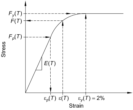
Figure description:
Stress-Strain Model at Temperature T
Stress vs. Strain Curve
Annotations
- (slope_label - position: Linear elastic region))
- (horizontal_reference_line - position: y = )))
- (horizontal_reference_line - position: y = )))
- (horizontal_reference_line - position: y = )))
- (vertical_reference_line - position: x = )))
- (vertical_reference_line - position: x = )))
- (vertical_reference_line - position: x = ))
| Strain | Stress |
|---|---|
| 0 | 0 |
| ) | ) |
| ) | ) |
| ) | ) |
| ) | ) |
Notes: The chart illustrates a material's stress-strain behavior at a given temperature T, featuring an initial linear elastic portion with slope E(T, transitioning into a curved region and finally reaching a perfectly plastic plateau at the yield stress F_y(T and yield strain of 2%.))
Fig. C-A-4.1. Parameters of idealized stress-strain curve at elevated temperatures (Takagi and Deierlein, 2007).
- (b) When
(C-A-4-13)
(c) When
(C-A-4-14)
(d) When
(C-A-4-15)
Table A-4.2.3 provides properties for Group 120 and 150 high-strength bolts at elevated temperatures expressed as strength retention factors, which are the ratios of bolt shear or tension strength at high temperatures with respect to the corresponding property at ambient temperature. The strength retention factors are based on a review of available experimental data (Gonzalez and Lange, 2009; Hanus et al., 2010, 2011; Kirby, 1995; Kodur et al., 2012; Li et al., 2001; Lou et al., 2010; Yu and Frank, 2009) and are consistent with values given in Eurocode 3 (CEN, 2005b). The available data indicates that retention factors are similar for both the shear and the tensile strength of bolts and are also similar for both Group 120 and 150 bolts. Consequently, Table A-4.2.3 specifies a single set of retention factors that are not, however, applicable to Group 144 or 200 bolts.
The strength of bolts depends on both temperature and temperature history. The strength retention factors given in Table A-4.2.3 assume the given temperature is the highest temperature to which the bolt has been exposed. For example, if a bolt
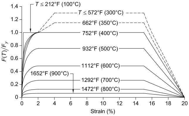
Figure description:
Normalized Stress-Strain Curves for Steel at Elevated Temperatures
Legend
- — color: black; symbol: Solid line
- — color: black; symbol: Dashed line
- — color: black; symbol: Dashed line
- — color: black; symbol: Solid line
- — color: black; symbol: Solid line
- — color: black; symbol: Solid line
- — color: black; symbol: Solid line
- — color: black; symbol: Solid line
- — color: black; symbol: Solid line
Annotations
- (text_label - position: Pointing to the plateau at F(T/Fy = 1.0)))
- (text_label - position: Pointing to the lowest curve with a plateau of ~0.06))
| Strain (%) | ) | ) | ) | ) | ) | ) | ) | ) | ) |
|---|---|---|---|---|---|---|---|---|---|
| 0 | 0.00 | 0.00 | 0.00 | 0.00 | 0.00 | 0.00 | 0.00 | 0.00 | 0.00 |
| 0.2 | 1.00 | 0.40 | 0.35 | 0.30 | 0.22 | 0.15 | 0.08 | 0.04 | 0.02 |
| 1.0 | 1.00 | 0.85 | 0.85 | 0.85 | 0.65 | 0.40 | 0.22 | 0.10 | 0.05 |
| 2.0 | 1.00 | 1.00 | 1.00 | 1.00 | 0.76 | 0.48 | 0.26 | 0.12 | 0.06 |
| 4.0 | 1.00 | 1.30 | 1.15 | 1.00 | 0.76 | 0.48 | 0.26 | 0.12 | 0.06 |
| 15.0 | 1.00 | 1.30 | 1.15 | 1.00 | 0.76 | 0.48 | 0.26 | 0.12 | 0.06 |
| 20.0 | 0.00 | 0.00 | 0.00 | 0.00 | 0.00 | 0.00 | 0.00 | 0.00 | 0.00 |
Notes: The Y-axis represents the ratio of stress at temperature T to the yield stress at room temperature (F(T/Fy. The X-axis represents strain as a percentage. The dashed lines for 300°C and 350°C indicate a strain-hardening region between 2% and 4% strain.))
Fig. C-A-4.2. Stress-strain relationships of structural steel at elevated temperatures with strain hardening per ECCS (2001).
is heated to 1,000°F (540°C), and this is the highest temperature the bolt has seen, the strength of the bolt at 1,000°F (540°C) can be computed as 42% of its normal room temperature value, as indicated in Table A-4.2.3. However, if the bolt has been heated to 1,600°F (870°C), for example, and then cools to 1,000°F (540°C), then the strength of the bolt at 1,000°F (540°C) may be less than 42% of the room temperature value. Limited data on the temperature history dependence of bolt strength is provided by Hanus et al. (2011). The temperature history dependence of bolt strength can be important when evaluating connection strength during the cooling stage of a fire. An additional important consequence of this behavior is that bolts can suffer a significant permanent loss of strength after being heated in a fire and then cooled to room temperature. This permanent loss of strength can be important when evaluating the condition of a steel structure after a fire. Information on the post-fire properties of high-strength bolts is reported by Yu and Frank (2009).
Appendix 4 does not currently include provisions for computing the elevated temperature strength of welds because of the lack of experimental data on elevated temperature properties of welds made using typical U.S. welding processes, procedures, and consumables. However, some guidance on the elevated temperature strength of welds is provided in Eurocode 3 (CEN, 2005b).
4.2.4 Structural Design Requirements
The resistance of the structural system in the design-basis fire may be determined by the following:
- (a) Structural analysis of individual elements where the effects of restraint to thermal expansion and bowing may be ignored but the reduction in strength and stiffness with increasing temperature is incorporated
- (b) Structural analysis of assemblies/subframes/frames where the effects of restrained thermal expansion and thermal bowing are considered by incorporating geometric and material nonlinearities
- (c) Global structural analysis where restrained thermal expansion, thermal bowing, material degradation, and geometric nonlinearity are considered
4.2.4a General Requirements
The requirement for general structural integrity is consistent with that appearing in Section 1.4 of ASCE/SEI 7 (ASCE, 2022). Structural integrity is the ability of the structural system to absorb and contain local damage or failure without developing into a progressive collapse that involves the entire structure or a disproportionately large part of it. Commentary Section C1.4 of ASCE/SEI 7 (ASCE, 2022) contains guidelines for the provision of general structural integrity.
Most typical structural steel connections will comply with the Chapter B tie-force requirements for structural integrity at ambient conditions without reinforcement or other modifications. The exceptions to this generalization are seated, single-angle, and bolted-welded double-angle (“knife”) connections (Gustafson, 2009). During a design-basis fire, large tensile and compressive forces develop in connections causing localized damage or failure of these and other types of connections (Agarwal
et al., 2014b; Fischer and Varma, 2015b; Selden et al., 2016; Fischer et al., 2017; Choe et al., 2020). This research indicates that additional design enhancements for ductility and resistance may be necessary to meet the performance objectives of the building during a design-basis fire.
Filled composite columns and shear walls subjected to fire loading can effectively sustain load during a fire exposure without benefit of any external protection for the steel. The concrete infill mass provides both an increased capacity for absorbing the heat caused by the fire and load-bearing strength to, thereby, extend the fire-resistance duration. However, these composite members will experience internal pressure build-up due to the steam emanating from concrete at elevated temperatures. The steam needs to be vented out to prevent the pressure build-up and its adverse effects on the members. The magnitude and rate of internal pressure build-up for a designbasis fire depends on the fire protection and moisture content of concrete infill. Anvari et al. (2020b) have developed a rational method that considers these factors and can be used to calculate the size and spacing of vent holes required to limit the internal pressure build-up to a specified value.
4.2.4b Strength Requirements and Deformation Limits
As structural elements are heated, their expansion is restrained by adjacent elements and connections. Material properties degrade with increasing temperature. Load transfer can occur from hotter elements to adjacent cooler elements. Excessive deformation may be of benefit in a fire as it allows release of thermally induced stresses. Deformation is acceptable once horizontal and vertical separation, as well as the overall load-bearing capacity of the structural system, is maintained.
Membrane action of concrete floor slabs exposed to fire has received growing international research attention. Beginning with the landmark Cardington fire tests conducted during the mid-1990s in the United Kingdom (Newman, 1999), this high-temperature strength mechanism has been identified as a fire-resistance design alternative for composite or reinforced concrete floor systems. The novel advantage of this membrane action design is that it permits the secondary infill steel floor beams to be left unprotected, because they are designed for strength and stiffness primarily at ambient conditions. The tradeoffs are that the concrete slab, all the fire-protected perimeter girders of the floor bays, and their end connections must have adequate strength and ductility to bridge over an entire floor bay and the severely thermally weakened infill beams, such that an adequate load path is maintained to transmit the gravity design loads of the floor bay. Agarwal and Varma (2014) and Agarwal et al. (2014b) have demonstrated that the presence of steel reinforcement greater than the minimum shrinkage reinforcement in the concrete slabs, and fire protection of the single-plate connections facilitates the redistribution of gravity loading through membrane action and reduces the risk of progressive collapse of the structure. Bailey (2004) provides further background and the design criteria for how to effectively mobilize membrane action at large vertical deflections. There have been numerous other published papers on this research advancement, such as Zhao et al. (2008), Huang et al. (2004), and Bednar et al. (2013).
4.2.4c Design by Advanced Methods of Analysis
Designs by advanced methods of analysis are permitted for all structures, loading, and fire scenarios. The load combination of Appendix 4, Section 4.1.4 (Equation A-4-1), and the design-basis fire from Appendix 4, Section 4.2.1, are used for such analyses. While the advanced methods may be used for simple regular structures and individual member evaluations, it is particularly applicable and useful for large or complex structures with irregularities in structural geometry, layout, and stiffness, or structures exposed to complex loading and design-basis fire scenarios.
In addition to the applicable requirements of Appendix 1, Section 1.3.1, numerical models used for advanced analysis may explicitly account for one or more of the following: (1) initiation, growth, and evolution of the design-basis fire scenario throughout the structure; (2) spatial and temporal variations of temperatures in the structure during the fire event; (3) modifications in stiffness and strength of structural materials, members, and connections with variations in temperature; (4) thermally induced deformations, including large deformation effects and time-dependent (creep) effects; and (5) uncertainties resulting from variabilities in material properties, modeling assumptions, and numerical analysis approaches. The advanced analysis models typically account for all considered limit states, including excessive deflections, member instability, cracking, spalling, connection ruptures, local failures, and overall global collapse.
For example, Agarwal and Varma (2014), Agarwal et al. (2014b), Fischer et al. (2019), and Gernay and Khorasoni (2020) conducted advanced analysis of 3D building structures while accounting for all potential limit states, namely, inelastic column buckling, composite slab cracking in tension, yielding of steel floor beams and slab reinforcement, and deformation and fracture of various shear connections. They used the Eurocode stress-strain-temperature relationships to model the deterioration in strength and stiffness with increasing temperature. Sample results from one of their advanced analyses are shown in Figure C-A-4.3.
Advanced methods of analysis consist of direct simulation of the thermal and structural behavior and performance of the structure for the design-basis event. Typically, this consists of a performance-based, probabilistic approach to conducting design that must demonstrate an adequate level of safety in order to be approved by the authority having jurisdiction. This can be achieved through a number of different approaches at the discretion of the designer, who has the responsibility to demonstrate that the performance objectives and intent of the building code are being upheld. In most cases, advanced methods of analysis do not result in calculated load effects (demands or required strengths) for members and connections that would then have to be compared with calculated resistances (available strengths) based on values given in Appendix 4, Section A4.2.4d(a) through (h), or other resources in the literature. However, if one were to use this approach to evaluate capacity and demand using the LRFD approach, -factors can be included by further reducing the and material data with the appropriate -factor.
Given the complexity of assumptions and numerical approaches used in design by the advanced methods of analyses, a peer-review team with applicable expertise and appropriate knowledge in this area may be engaged to review the following: (1) the calibration, benchmarking, or verification of the various modeling assumptions and approaches used, and (2) the results from the advanced analyses with respect to fundamental understanding of behavior and overall performance objectives established for the structure. It is important to note that some failure modes may not be simulated accurately, if at all, with advanced analysis methods; for example, concrete slab perforation, creep-related buckling, material behavior, and fracture in the cooling phase, etc. The results from such advanced analyses should, therefore, be treated with caution and engineering judgment.
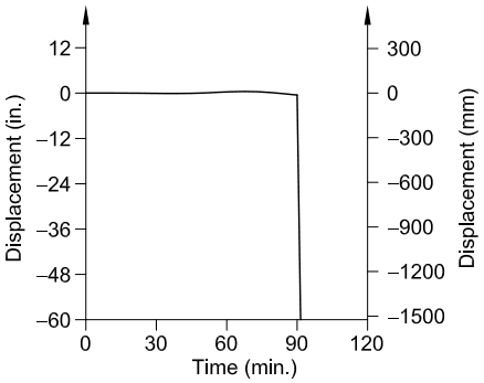
Figure description:
| Time (min.) | Displacement (in.) | Displacement (mm) |
|---|---|---|
| 0 | 0.0 | 0 |
| 15 | 0.0 | 0 |
| 30 | 0.0 | 0 |
| 45 | 0.0 | 0 |
| 60 | 0.5 | 12.5 |
| 75 | 1.0 | 25 |
| 85 | 0.5 | 12.5 |
| 89.9 | 0.0 | 0 |
| 90.0 | -60.0 | -1500 |
Notes: The chart shows a displacement that remains near zero for the first 90 minutes, with a slight positive peak around 75 minutes, followed by a sudden vertical drop to -60 inches (-1500 mm at exactly 90 minutes.)
(a) Interior gravity column failure displacement history
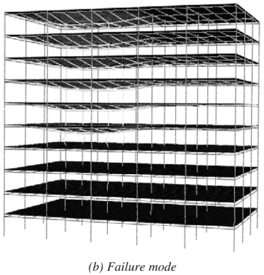
Figure description:
- Subject: 3D structural model of a 10-story building illustrating a failure mode.
- Event: Simulation of interior gravity column failure caused by a design fire.
- Key Observation: Pronounced sagging and downward deflection of floor slabs in the central bay of the upper floors.
- Structural Impact: The deformation is localized to the central column line, with the lower four floors remaining relatively undeformed.
Fig. C-A-4.3. Advanced analysis of 3D building for design fire.
Specification for Structural Steel Buildings, August 1, 2022 AMERICAN INSTITUTE OF STEEL CONSTRUCTION
4.2.4d Design by Simple Methods of Analysis
Design by simple methods of analysis permits two structural analysis approaches. As discussed in Chicchi and Varma (2022), engineering judgment is required to select the more reasonable, conservative, and appropriate approach for a structure, loading, and fire scenario.
The first approach may be more applicable to the stability and design of members, for example, columns, simply supported beams, composite girders, etc., in regular gravity frames. This approach assumes that the load effects (demands or required strengths) for the fire loading combination can be calculated using analyses similar to ambient conditions in accordance with Specification Section C1.2 or C2 with no additional changes in support or restraint conditions for individual members throughout the fire scenario. The factored resistance (available strengths) for individual members can be calculated using Appendix 4, Sections 4.2.4d(a) through (h).
The second approach may be more appropriate to the stability design of irregular structural frames with discontinuities in structural plan, geometry, or stiffness. This approach assumes that the load effects (demands/required strengths) for the fire loading combination can be calculated using elastic analysis methods of Specification Sections C2 or Appendix 1, Section 1.2, considering the following: (1) appropriate modifications to account for the effects of elevated temperature on member and connection stiffness, as applicable, and (2) thermal deformation effects due to maximum elevated temperatures and thermal gradients. The factored resistance (available strength) for members can be calculated using Section 4.2.4d(a) through (h), as applicable, or using other applicable resources in the literature [for example, Agarwal et al. (2014a) and Garlock and Quiel (2008)].
Even for fire design, all compactness and slenderness limits can be evaluated using ambient temperature values of and . The Eurocode 4 (CEN, 2005d) provisions indicate that the plastic bending strength of composite beams during a fire exposure can be achieved for all nonslender shapes, which implies that for composite beams, the limiting width-to-thickness ratios can be the maximum AISC values for webs, , and for flanges, .
Takagi and Deierlein (2007) have shown that the standard strength equations of this Specification at ambient temperature, with steel properties, , and , reduced for elevated temperatures, can overestimate considerably the strengths of members that are sensitive to stability effects. Special high-temperature equations developed by Takagi and Deierlein (2007) more accurately represent the strength of unrestrained compression members subjected to flexural buckling and flexural members subjected to lateral-torsional buckling. As shown in Figure C-A-4.4, these equations, first introduced in the 2010 AISC Specification (AISC, 2010), are much more accurate in comparison to equations from the ECCS (2001) and to detailed finite element method analyses (represented by the square symbol in the figure), which have been validated against test data.
The stability of steel structures under fire loading is governed by the fire resistance of gravity columns because they are most likely to reach critical temperatures and structural failure due to high utilization ratios (Agarwal and Varma, 2011, 2014).
The fire resistance of gravity columns may be improved due to the rotational restraints offered by cooler columns in the stories above and below. This reduction in column slenderness, , may be calculated using Equation A-4-10 or A-4-10M. The column in the heated story has a reduced flexural stiffness, , due to fire exposure. In the case of a one-story fire, the cooler columns above and below the heated column would have the larger intact , which provides rotational restraint and decreases column slenderness of the heated column. Figure C-A-4.5 shows this reduction in with increasing temperature for columns with rotational restraints at both ends and one end only.
Compression members subjected to uniform heating have greater heat flux from all sides than members subjected to nonuniform heating. As a result, compression members subjected to uniform heating typically reach their failure temperatures much earlier than members subjected to nonuniform heating. Uniform heating will be the governing case for most fire scenarios (Agarwal et al., 2014a) in terms of time to failure.
Thermal gradients due to nonuniform heating reduce the axial load capacity of compression members due to elevated temperatures, bowing deformations resulting from uneven thermal expansion, and asymmetry in the column cross section resulting from uneven degradation of material properties (yield stress and elastic modulus). Several researchers have discussed these effects and proposed alternative design methods for columns with thermal gradients. Agarwal et al. (2014a) and Choe et al. (2016) conducted experimental and numerical studies to develop and verify design equations for compression members with thermal gradients. The parameters included in the study were member length, cross section, and axial loading magnitude. Three different heating scenarios were considered: uniform heating, thermal gradient along the flanges, and thermal gradient along the web. The studies indicated that columns subjected to uniform heating have much greater heat influx, and therefore, reach higher average temperatures faster than columns exposed to nonuniform heating. In most cases, uniformly heated columns reached their failure temperature earlier than nonuniformly heated columns with thermal gradients; exceptions were slender
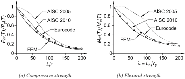
Figure description:
Comparison of Compressive and Flexural Strength Models
(a Compressive strength
Legend
- FEM — color: black; symbol: Solid line with square/circle markers
- AISC 2005 — color: black; symbol: Dotted line
- AISC 2010 — color: black; symbol: Dashed line
- Eurocode — color: black; symbol: Dash-dot line
| L/r | FEM | AISC 2005 | AISC 2010 | Eurocode |
|---|---|---|---|---|
| 0 | 1.00 | 1.00 | 1.00 | 1.00 |
| 20 | 0.81 | 0.98 | 0.84 | 0.82 |
| 40 | 0.60 | 0.92 | 0.62 | 0.59 |
| 60 | 0.46 | 0.81 | 0.48 | 0.46 |
| 80 | 0.36 | 0.66 | 0.38 | 0.36 |
| 100 | 0.28 | 0.49 | 0.31 | 0.29 |
| 120 | 0.22 | 0.37 | 0.25 | 0.23 |
| 140 | 0.17 | 0.27 | 0.20 | 0.18 |
| 160 | 0.13 | 0.20 | 0.16 | 0.14 |
| 180 | 0.11 | 0.14 | 0.13 | 0.11 |
| 200 | 0.09 | 0.11 | 0.11 | 0.10 |
(b Flexural strength
Legend
- FEM — color: black; symbol: Solid line with square markers
- AISC 2005 — color: black; symbol: Dotted line
- AISC 2010 — color: black; symbol: Dashed line
- Eurocode — color: black; symbol: Dash-dot line
| lambda = Lb/ry | FEM | AISC 2005 | AISC 2010 | Eurocode |
|---|---|---|---|---|
| 0 | 1.00 | 1.00 | 1.00 | 1.00 |
| 20 | 0.81 | 1.00 | 0.82 | 0.81 |
| 40 | 0.66 | 0.98 | 0.66 | 0.66 |
| 60 | 0.52 | 0.89 | 0.52 | 0.53 |
| 80 | 0.44 | 0.82 | 0.43 | 0.44 |
| 100 | 0.36 | 0.74 | 0.36 | 0.35 |
| 120 | 0.29 | 0.52 | 0.29 | 0.28 |
| 140 | 0.24 | 0.38 | 0.24 | 0.23 |
| 160 | 0.20 | 0.28 | 0.20 | 0.22 |
| 180 | 0.18 | 0.23 | 0.18 | 0.21 |
| 200 | 0.15 | 0.20 | 0.15 | 0.20 |
Notes: The charts compare normalized compressive and flexural strengths against slenderness ratios using Finite Element Method (FEM and various design standards (AISC 2005, AISC 2010, Eurocode.))
Fig. C-A-4.4. Comparison of compressive and flexural strengths at 500°C (930°F) (Takagi and Deierlein, 2007).
columns with very high axial compression (more than 50% of ambient capacity). The design strength of such columns can be calculated using equations presented by Agarwal et al. (2014a). These equations quantify the effects of elevated temperature, bowing, and cross-section asymmetry mentioned earlier. They were verified using the results of large-scale tests and numerical parametric studies.
Equation A-4-15 is used to calculate for structural members subjected to flexure when . This equation is a modification of Equation F2-4 used to calculate the available flexural strength at ambient temperatures. These equations assume a constant value for shear modulus, , which does not vary with temperature.
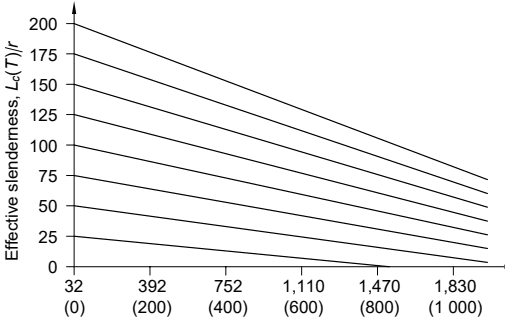
Figure description:
Effective Slenderness as a Function of Temperature Variation of effective slenderness ratio with increasing temperature for various initial values.
Effective slenderness, versus Temperature
Legend
- Initial slenderness = 200 — color: black; symbol: Solid line
- Initial slenderness = 175 — color: black; symbol: Solid line
- Initial slenderness = 150 — color: black; symbol: Solid line
- Initial slenderness = 125 — color: black; symbol: Solid line
- Initial slenderness = 100 — color: black; symbol: Solid line
- Initial slenderness = 75 — color: black; symbol: Solid line
- Initial slenderness = 50 — color: black; symbol: Solid line
- Initial slenderness = 25 — color: black; symbol: Solid line
| Temperature (°F) | Temperature (°C) | Lc(T/r (Initial=200)) | Lc(T/r (Initial=175)) | Lc(T/r (Initial=150)) | Lc(T/r (Initial=125)) | Lc(T/r (Initial=100)) | Lc(T/r (Initial=75)) | Lc(T/r (Initial=50)) | Lc(T/r (Initial=25)) |
|---|---|---|---|---|---|---|---|---|---|
| 32 | 0 | 200 | 175 | 150 | 125 | 100 | 75 | 50 | 25 |
| 392 | 200 | 175 | 153 | 131 | 109 | 87 | 65 | 44 | 21 |
| 752 | 400 | 148 | 130 | 110 | 91 | 73 | 54 | 35 | 16 |
| 1,110 | 600 | 122 | 107 | 91 | 75 | 59 | 44 | 28 | 11 |
| 1,470 | 800 | 97 | 84 | 71 | 58 | 45 | 31 | 17 | 2 |
| 1,830 | 1,000 | 72 | 60 | 49 | 38 | 27 | 16 | 5 | null |
Notes: The x-axis displays temperature in degrees Fahrenheit with degrees Celsius in parentheses. The y-axis represents the effective slenderness ratio . Multiple series are plotted starting from different initial slenderness values at .)
Temperature, °F (°C)
(a) Rotational restraint at both ends
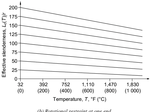
Figure description:
Effective slenderness, Lc(T/r versus Temperature, T (b Rotational restraint at one end
Effective slenderness vs Temperature
Legend
- Initial slenderness = 200 — color: black; symbol: Solid line
- Initial slenderness = 175 — color: black; symbol: Solid line
- Initial slenderness = 150 — color: black; symbol: Solid line
- Initial slenderness = 125 — color: black; symbol: Solid line
- Initial slenderness = 100 — color: black; symbol: Solid line
- Initial slenderness = 75 — color: black; symbol: Solid line
- Initial slenderness = 50 — color: black; symbol: Solid line
- Initial slenderness = 25 — color: black; symbol: Solid line
| Temperature (°C) | Temperature (°F) | Effective slenderness (initial 200)) | Effective slenderness (initial 175)) | Effective slenderness (initial 150)) | Effective slenderness (initial 125)) | Effective slenderness (initial 100)) | Effective slenderness (initial 75)) | Effective slenderness (initial 50)) | Effective slenderness (initial 25)) |
|---|---|---|---|---|---|---|---|---|---|
| 0 | 32 | 200.0 | 175.0 | 150.0 | 125.0 | 100.0 | 75.0 | 50.0 | 25.0 |
| 200 | 392 | 192.0 | 168.0 | 144.0 | 120.0 | 96.0 | 72.0 | 48.0 | 24.0 |
| 400 | 752 | 182.0 | 159.3 | 136.5 | 113.8 | 91.0 | 68.3 | 45.5 | 22.8 |
| 600 | 1110 | 168.0 | 147.0 | 126.0 | 105.0 | 84.0 | 63.0 | 42.0 | 21.0 |
| 800 | 1470 | 156.0 | 136.5 | 117.0 | 97.5 | 78.0 | 58.5 | 39.0 | 19.5 |
| 1000 | 1830 | 144.0 | 126.0 | 108.0 | 90.0 | 72.0 | 54.0 | 36.0 | 18.0 |
Notes: The chart shows multiple data series, each representing a different initial effective slenderness value at 0°C (32°F. The lines show how effective slenderness decreases with increasing temperature under the condition of rotational restraint at one end.)
(b) Rotational restraint at one end
Fig. C-A-4.5. Effects of rotational restraints on column slenderness as a function of elevated temperature (from Equation A-4-10).
In reality, as shown by G(T) in Table A-4.2.1, the shear modulus varies with temperature. The alternative equation mentioned in a User Note in Section F2.2 may be used to incorporate this change in shear modulus due to elevated temperatures.
The equations for compression strength of composite columns and composite plate shear walls at elevated temperatures have been developed based on parametric studies conducted by Anvari et al. (2020a) and Wazalwar et al. (2020). Wazalwar et al. (2020) developed a numerical tool to evaluate the fire performance of filled columns. The tool was benchmarked using existing experimental data for filled composite columns subjected to fire loading. The authors conducted a study to evaluate the effect of parameters, such as the aspect ratio (length-to-width ratio), section slenderness, and concrete and steel strengths on the strength degradation at elevated temperatures. Figure C-A-4.6 shows the comparison of Equation A-4-11 with the parametric study data from the tool. Equation A-4-11 provides a lower-bound estimate of filled composite column compression strength.
Anvari et al. (2020a) conducted detailed finite element analyses for composite plate shear walls, using models validated against experimental data. Figure C-A-4.7 shows the comparison of Equation A-4-12 with the finite element data. The data plotted include planar walls with a length-to-thickness ratio of 3 and corresponding unit width column strips (with no flange plates). Equation A-4-12 provides a lower-bound estimate of composite plate shear wall compression strength.
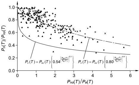
Figure description:
Variation of normalized power with pressure ratio
Normalized power ratio vs pressure ratio
Legend
- Triangles — color: black; symbol: triangle
- Circles — color: black; symbol: circle
- Crosses — color: black; symbol: cross (x
- Squares — color: black; symbol: small square
- Solid Line — color: black; symbol: Solid line
- Dashed Line — color: black; symbol: Long-dashed line
Annotations
- P_n(T = P_no(T { 0.54 [P_no(T / P_e(T^-0.3 } (text_label - position: x ≈ 2.2, y ≈ 0.2; points to solid line)))))
- P_n(T = P_no(T { 0.80 [P_no(T / P_e(T^-0.3 } (text_label - position: x ≈ 4.5, y ≈ 0.2; points to dashed line)))))
| P_no(T / P_e(T)) | Series | P_n(T / P_no(T)) |
|---|---|---|
| 0.05 | Triangles | 0.91 |
| 0.10 | Triangles | 0.98 |
| 0.20 | Triangles | 0.77 |
| 0.30 | Triangles | 0.55 |
| 0.40 | Triangles | 0.85 |
| 0.50 | Triangles | 0.99 |
| 0.60 | Triangles | 0.68 |
| 0.70 | Triangles | 0.98 |
| 0.80 | Triangles | 0.81 |
| 1.00 | Triangles | 0.71 |
| 1.50 | Triangles | 0.54 |
| 2.00 | Triangles | 0.98 |
| 3.00 | Triangles | 0.40 |
| 4.20 | Triangles | 0.28 |
| 4.60 | Triangles | 0.32 |
| 5.70 | Triangles | 0.37 |
| 0.50 | Circles | 0.90 |
| 1.00 | Circles | 0.85 |
| 1.50 | Circles | 0.92 |
| 2.00 | Circles | 0.78 |
| 2.50 | Circles | 0.65 |
| 3.00 | Circles | 0.71 |
| 4.00 | Circles | 0.50 |
| 0.70 | Crosses | 0.87 |
| 1.00 | Crosses | 0.92 |
| 1.50 | Crosses | 0.71 |
| 2.00 | Crosses | 0.71 |
| 3.10 | Crosses | 0.63 |
| 4.70 | Crosses | 0.59 |
| 1.00 | Squares | 1.00 |
| 1.40 | Squares | 0.95 |
| 2.20 | Squares | 0.85 |
| 3.80 | Squares | 0.67 |
| 5.10 | Squares | 0.53 |
| 0.10 | Solid Line | 0.75 |
| 0.50 | Solid Line | 0.55 |
| 1.00 | Solid Line | 0.45 |
| 2.00 | Solid Line | 0.38 |
| 4.00 | Solid Line | 0.30 |
| 6.00 | Solid Line | 0.25 |
| 0.10 | Dashed Line | 0.95 |
| 0.50 | Dashed Line | 0.88 |
| 1.00 | Dashed Line | 0.80 |
| 2.00 | Dashed Line | 0.71 |
| 4.00 | Dashed Line | 0.52 |
| 6.00 | Dashed Line | 0.39 |
Notes: The y-axis represents P_n(T / P_no(T and the x-axis represents P_no(T / P_e(T. The trend lines are defined by power laws as shown in the annotations. The scatter points likely represent different datasets or experimental conditions.))))
• Series 1: Aspect ratio • Series 2: Section slenderness • Series 3: Steel strength • Series 4: Concrete strength
Fig. C-A-4.6. Determination of compression strength of filled composite columns with Equation A-4-11 compared to numerical tool (Anvari et al., 2020a; Wazalwar et al., 2020).
For composite plate shear walls, the simplified analyses can be conducted per unit width of the wall and one-dimensional heat-transfer equations can be used to model the thermal response. The unit width method for shear walls is conservative and can be used for different configurations of the walls, including planar walls and C-shaped walls (Anvari et al., 2020a).
For composite beams, Selden and Varma (2016) developed and benchmarked numerical models to determine their flexural strength at elevated temperatures, , while considering the distribution of temperatures over the depth of the composite section, the degree or percentage of composite action in the section, member length, and the effects of elevated temperature on the material stiffness and strength of the steel beam, concrete slab, steel reinforcement (if any), and the shear force-slip behavior of the steel anchors. The results of comprehensive parametric analyses conducted by Selden (2014) were used to develop Equation A-4-20 and the retention factors in Table A-4.2.4.
A simplified thermal gradient profile along the depth of a composite beam has been prescribed when lumped heat capacity analysis is used to compute the single maxi- mum temperature in the beam’s bottom flange. The intent of this provision was to offer a convenient and conservative alternative to a more rigorous determination of
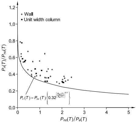
Figure description:
Normalized Axial Load Capacity of Masonry Walls and Columns under Fire Conditions
vs.
Legend
- Wall — color: grey; symbol: Diamond
- Unit width column — color: black; symbol: Square
Annotations
- (text_label - position: y = 0.32 * x^(-0.3))))))
| )) | Wall ())) | Unit width column ())) | Predicted Curve ())) |
|---|---|---|---|
| 0.05 | 0.787 | ||
| 0.1 | 0.79 | 0.61 | 0.638 |
| 0.15 | 0.65 | 0.565 | |
| 0.2 | 0.78 | 0.58 | 0.519 |
| 0.25 | 0.59 | 0.485 | |
| 0.3 | 0.55 | 0.459 | |
| 0.35 | 0.55 | 0.439 | |
| 0.4 | 0.57 | 0.56 | 0.422 |
| 0.5 | 0.68 | 0.394 | |
| 0.6 | 0.45 | 0.373 | |
| 0.7 | 0.44 | 0.37 | 0.356 |
| 0.75 | 0.4 | 0.349 | |
| 0.8 | 0.38 | 0.342 | |
| 0.85 | 0.55 | 0.46 | 0.336 |
| 0.9 | 0.38 | 0.41 | 0.330 |
| 1.0 | "0.39, 0.56" | 0.320 | |
| 1.1 | 0.41 | 0.45 | 0.311 |
| 1.25 | 0.36 | 0.31 | 0.299 |
| 1.3 | 0.65 | 0.31 | 0.295 |
| 1.35 | 0.44 | 0.292 | |
| 1.4 | 0.46 | 0.35 | 0.289 |
| 1.5 | 0.38 | 0.283 | |
| 1.65 | 0.37 | 0.275 | |
| 1.75 | 0.31 | 0.270 | |
| 1.9 | 0.29 | 0.264 | |
| 2.0 | 0.34 | 0.31 | 0.260 |
| 2.05 | 0.3 | 0.258 | |
| 2.1 | 0.38 | 0.3 | 0.256 |
| 2.15 | 0.35 | 0.254 | |
| 2.2 | 0.32 | 0.253 | |
| 2.3 | 0.33 | 0.250 | |
| 2.4 | 0.36 | 0.246 | |
| 3.0 | 0.230 | ||
| 4.0 | 0.211 | ||
| 5.0 | 0.197 |
Notes: The data table includes estimated values for the 'Wall' and 'Unit width column' series from the scatter plot, as well as calculated points for the 'Predicted Curve' based on the provided empirical equation. Multiple points for the same x-coordinate are listed within quotes in the table cell.
Fig. C-A-4.7. Determination of compression strength of composite plate shear walls and unit strip columns with Equation A-4-12 compared to finite element analysis (Anvari et al., 2020a).
the steel temperatures from thermal analysis and fire tests. Thus, a composite beam’s temperature profile may be based on analysis or experimental data in lieu of this default thermal gradient.
The design strength for structural steel members and connections is calculated as , in which is the nominal strength when the deterioration in strengthat elevated temperature is taken into account, and is the resistance factor. The nominal strength is determined from Chapters C through K and Appendix 4, using material strength and stiffnesses at elevated temperatures defined in Tables A-4.2.1, A-4.2.2, and A-4.2.3. For limit states governed by steel yielding or rupture, the ambient temperature equations for nominal strength are used with elevated temperature material properties from Appendix 4, Section 4.2.3, and the corresponding tables. For limit states governed by buckling or instability, equations for nominal strength are provided in this section. For example, nominal strength equations are provided for design for compression and for flexure governed by lateral-torsional buckling.
While ECCS (2001) and Eurocode 1 (CEN, 1991) specify partial material factors as equal to 1.0 for “accidental” limit states, the uncertainties in strength at elevated temperatures are substantial and in some cases are unknown. Research is continuing on this topic. In the interim, ambient resistance factors should be used when determining design strength.
4.2.4e Design by Critical Temperature Method
The critical temperature approach provides an alternative method to the member resistance method in Appendix 4, Section 4.2.4d. This approach only considers uniform heating of individual members with wide-flange rolled shapes that have nonslender elements as defined in Section B4. Local buckling effects at elevated temperatures are thus precluded.
For yielding of tension members or continuously braced beams, the critical temperature is calculated based on the yield stress at elevated temperature in accordance with Eurocode 3 (CEN, 2005b) as shown in Figure C-A-4.8(a). Its formulation is the same as the mathematical relationship of the temperatures corresponding to retention factors for yield stress, , in Table A-4.2.1. This relationship holds true for ratios greater than 0.01 . Thus, this relationship applies to most cases, as load ratios or less than 0.01 are highly unlikely due to the member self-weight.
For flexural buckling of compression members, the critical temperature calculated using Equation A-4-22 (A-4-22M) correlates closely with critical temperatures back-calculated using Equation A-4-9 for load ratios less than 0.6 (Sauca et al., 2021). As shown in Figure C-A-4.8(b), Equation A-4-22 (A-4-22M) provides a conservative lower bound (16% lower on average) relative to the column test data at load ratios greater than 0.3 (Sauca et al., 2021).