C-C2C2 Calculation of required strengths
PDF page 403 · AISC 360-22
Analysis to determine required strengths in accordance with this section and the assessment of member and connection available strengths in accordance with Section C3 form the basis of the direct analysis method of design for stability. This method is useful for the stability design of all structural steel systems, including moment frames, braced frames, shear walls, and combinations of these and similar systems (AISC-SSRC, 2003a). While the precise formulation of this method is unique to the Specification, some of its features are similar to those found in other major design specifications around the world, including the Eurocodes, the Australian standard, the Canadian standard, and ACI 318 (ACI, 2019).
The direct analysis method allows a more accurate determination of the load effects in the structure through the inclusion of the effects of geometric imperfections and stiffness reductions directly within the structural analysis. This also allows the use of in calculating the in-plane column strength, , within the beam-column interaction equations of Chapter H. This is a significant simplification in the design of steel moment frames and combined systems. Verification studies for the direct analysis method are provided by Deierlein et al. (2002), Maleck and White (2003), and Martinez-Garcia and Ziemian (2006).
C2.1 General Analysis Requirements
Deformations to be Considered in the Analysis. It is required that the analysis consider flexural, shear, and axial deformations, and all other component and connection deformations that contribute to the displacement of the structure. However, it is important to note that "consider" is not synonymous with "include," and some deformations can be neglected after rational consideration of their likely effect. For example, the in-plane deformation of a concrete-on-steel deck floor diaphragm in an office building usually can be neglected, but that of a cold-formed steel roof deck in a large warehouse with widely spaced lateral force-resisting elements usually cannot. As another example, shear deformations in beams and columns in a low-rise moment frame usually can be neglected, but this may not be true in a high-rise framed-tube system with relatively deep members and short spans. For such frames, the use of rigid offsets to account for member depths may significantly overestimate frame stiffness and consequently underestimate second-order effects due to high shear stresses within the panel zone of the connections. For example, Charney and Johnson (1986) found that for the range of columns and beam sizes they studied, the deflections of a subassembly modeled using centerline dimensions could vary from an overestimation of to an underestimation of when compared to a finite element model. Charney and Johnson conclude that analysis based on centerline dimensions may either underestimate or overestimate drift, with results depending on the span of the girder and on the web thickness of the column.
Second-Order Effects. The direct analysis method includes the basic requirement to calculate the internal load effects using a second-order analysis that accounts for both and effects (see Figure C-C2.1). effects are the effects of loads acting on the displaced location of joints or member-end nodes in a structure. effects are the effect of loads acting on the deflected shape of a member between joints or member-end nodes.
Many, but not all, modern commercial structural analysis programs are capable of accurately and directly modeling all significant and second-order effects. Programs that accurately estimate second-order effects typically solve the governing differential equations either through the use of a geometric stiffness approach (McGuire et al., 2000; Ziemian, 2010) or the use of stability functions (Chen and Lui, 1987). What is, and just as importantly what is not, included in the analysis should be verified by the user for each particular program. Some programs neglect effects in the analysis of the structure, and because this is a common approximation that is permitted under certain conditions, it is discussed at the end of this section.
Methods that modify first-order analysis results through second-order multipliers are permitted. The use of the and multipliers provided in Appendix 8 is one such method. The accuracy of other methods should be verified.
Analysis Benchmark Problems. The following benchmark problems are recommended as a first-level check to determine whether an analysis procedure meets the requirements of a and second-order analysis adequate for use in the direct analysis method (and the effective length method in Appendix 7). Some secondorder analysis procedures may not include the effects of on the overall response of the structure. These benchmark problems are intended to reveal whether or not these effects are included in the analysis. It should be noted that in accordance with the requirements of Section C2.1(b), it is not always necessary to include effects in the second-order analysis (additional discussion of the consequences of neglecting these effects will follow).
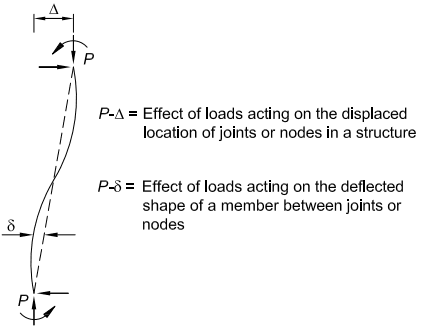
Figure description:
Key Information:
- Subject: and effects in beam-columns.
- Definition: The effect of loads acting on the displaced location of joints or nodes in a structure. Represented visually by the global horizontal displacement ( of the top node relative to the bottom.
- Definition: The effect of loads acting on the deflected shape of a member between joints or nodes. Represented visually by the local curvature and displacement ( of the member relative to its chord.
- Forces: Shows axial loads (, horizontal point loads, and moments acting on a vertically oriented member.
- Visual Elements: A dashed line represents the chord between nodes, while a solid curved line represents the deflected shape of the member.
Fig. C-C2.1. P-Δ and P-δ effects in beam-columns.
The benchmark problem descriptions and solutions are shown in Figures C-C2.2 and C-C2.3. Proportional loading is assumed and axial, flexural, and shear deformations are included. Case 1 is a simply supported beam-column subjected to an axial load concurrent with a uniformly distributed transverse load between supports. This problem contains only effects because there is no translation of one end of the member relative to the other. Case 2 is a fixed-base cantilevered beam-column subjected to an axial load concurrent with a lateral load at its top. This problem contains both and effects. In confirming the accuracy of the analysis method, both moments and deflections should be checked at the locations shown for the various levels of axial load on the member and in all cases should agree within and , respectively.
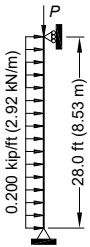
Figure description:
Structural Component: Simply supported beam-column (Case 1 Length: 28.0 ft (8.53 m Axial Load: Point load applied at the top Transverse Load: Uniformly distributed load of 0.200 kip/ft (2.92 kN/m Boundary Conditions: Pin support at the base and roller support at the top
| Axial Force, P (kips) | 0 | 150 | 300 | 450 |
|---|---|---|---|---|
| Mmid (kip-in.) | 235 [235] | 270 [269] | 316 [313] | 380 [375] |
| Δmid (in.) | 0.202 [0.197] | 0.230 [0.224] | 0.269 [0.261] | 0.322 [0.311] |
| Axial Force, P×10-3 (N) | 0 | 667 | 1,330 | 2,000 |
|---|---|---|---|---|
| Mmid×10-6 (N-mm) | 26.6 [26.6] | 30.5 [30.4] | 35.7 [35.4] | 42.9 [42.4] |
| Δmid (mm) | 5.13 [5.00] | 5.84 [5.69] | 6.83 [6.63] | 8.18 [7.90] |
Major-axis bending Analyses include axial, flexural, and shear deformations. W14x48 (W360x72) [Values in brackets] exclude shear deformations. E = 29,000 ksi (200 000 MPa)
Fig. C-C2.2. Benchmark problem Case 1.
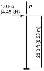
Figure description:
Benchmark problem Case 1 structural diagram:
- Vertical member height: (
- Support: Fixed base
- Applied loads at the top:
- Vertical axial load:
- Horizontal lateral load: (
| |||||||||||||||
|
Major-axis bending W14x48 (W360x72) E = 29,000 ksi (200 000 MPa)
Analyses include axial, flexural, and shear deformations. [Values in brackets] exclude shear deformations.
Fig. C-C2.3. Benchmark problem Case 2.
Given that there are many attributes that must be studied to confirm the accuracy of a given analysis method for routine use in the design of general framing systems, a wide range of benchmark problems should be employed. Several other targeted analysis benchmark problems can be found in White et al. (2021), Chen and Lui (1987), and McGuire et al. (2000). When using benchmark problems to assess the correctness of a second-order procedure, the details of the analysis used in the benchmark study, such as the number of elements used to represent the member and the numerical solution scheme employed, should be replicated in the analysis used to design the actual structure. Because the ratio of design load to elastic buckling load is a strong indicator of the influence of second-order effects, benchmark problems with such ratios on the order of 0.6 to 0.7 should be included.
Effect of Neglecting P-δ. A common type of approximate analysis is one that captures only effects due to member end translations (for example, interstory drift) but fails to capture effects due to curvature of the member relative to its chord. This type of analysis is referred to as a analysis. Where effects are significant, errors arise in approximate methods that do not accurately account for the effect of moments on amplification of both local ( ) and global ( ) displacements, and corresponding internal moments. These errors can occur both with second-order computer analysis programs and with the and amplifiers. For instance, the modifier in Equation A-8-7 is an adjustment factor that approximates the effects of (due to column curvature) on the overall sidesway displacements, , and the corresponding moments. For regular rectangular moment frames, a single-element-per-member analysis is equivalent to using the amplifier of Equation A-8-6 with , and hence, such an analysis neglects the effect of on the response of the structure.
Section C2.1(b) indicates that a -only analysis (one that neglects the effect of deformations on the response of the structure) is permissible for typical building structures when the ratio of second-order drift to first-order drift is less than 1.7 and no more than one-third of the total gravity load on the building is on columns that are part of moment-resisting frames. The latter condition is equivalent to an value of 0.95 or greater. When these conditions are satisfied, the error in lateral displacement from a -only analysis typically will be less than . However, when the effect in one or more members is large (corresponding to a multiplier of more than about 1.2), use of a -only analysis may lead to larger errors in the nonsway moments in components connected to the high- members.
The engineer should be aware of this possible error before using a -only analysis in such cases. For example, consider the evaluation of the fixed-base cantilevered beam-column shown in Figure C-C2.4 using the direct analysis method. The sidesway displacement amplification factor is 3.83 and the base moment amplifier is 3.32 , giving .
For the loads shown, the beam-column strength interaction according to Equation H1-1a is equal to 1.0. The sidesway displacement and base moment amplification determined by a single-element analysis, which ignores the effect of on the response of the structure, is 2.55 , resulting in an estimated . -an error of relative to the more accurate value of and a beam-column interaction value of 0.91 .
effects can be captured in some (but not all) -only analysis methods by subdividing the members into multiple elements. For this example, three equal-length analysis elements are required to reduce the errors in the second-order base moment and sidesway displacement to less than and , respectively.
It should be noted that, in this case, the unconservative error that results from ignoring the effect of on the response of the structure is removed through the use of Equation A-8-8. For the loads shown in Figure C-C2.4, Equations A-8-6 and A-8-7 with give a amplifier of 3.52 . This corresponds to . in the preceding example; approximately over that determined from a computational second-order analysis that includes both and effects.
For sway columns with nominally simply supported base conditions, the errors in the second-order internal moment and in the second-order displacements from a -only analysis are generally smaller than and , respectively, when ,
where
- (LRFD)
- = 1.6 (ASD)
- required axial force, ASD or LRFD, kips (N)
- if the analysis uses nominal stiffness, kips (N)
For sway columns with rotational restraint at both ends of at least if the analysis uses nominal stiffness, or if the analysis uses a flexural stiffness reduction of , the errors in the second-order internal moments and displacements from a -only analysis are generally smaller than and , respectively, when .
| Pu = 440 kips (1.96×10⁶ N) | Pu/Py = 0.50, τ = 1.0 | |
| H = Hu + Ni = 1.45 kips + 0.002(440 kips) = 2.33 kips (10 400 N) | E = 0.80τ(29,000 ksi) = 23,200 ksi (160 000 MPa) | |
| G = E/2(1+ν) = 8,920 ksi (61 500 MPa) | ||
| <ins>Computational P-Δ and P-δ analysis:</ins> | ||
| Δ2nd = 2.22 in. (56.4 mm) | ||
| 15.0 ft (4.6 m) | Mu = 1,390 kip-in. (157×106 N-mm) | |
| Major-axis bending Fully braced out-of-plane W10×60 (W250×89) Fy = 50 ksi (345 MPa) Include axial, flexural, and shear deformations | Pu/φcPn + (8/9)(Mu/φbMn) = 1.00 | |
| <ins>Single-element P-Δ analysis:</ins> | ||
| Δ1st = 0.580 in. (15 mm) | ||
| M1st = HL = 419 kip-in. (47.3×10⁶ N-mm) | ||
| 1 / [1-[Pu/(HL/Δ1st)]] = 2.55 | ||
| MP-Δ = 2.55M1st = 1,070 kip-in. (121×106 N-mm) | ||
| Pu/φcPn + (8/9)(MP-Δ/φbMn) = 0.910 |
Fig. C-C2.4. Illustration of potential errors associated with the use of a single-element-per-member P-Δ analysis.
For members subjected predominantly to nonsway end conditions, the errors in the second-order internal moments and displacements from a -only analysis are generally smaller than and , respectively, when .
In meeting these limitations for use of a -only analysis, it is important to note that in accordance with Section C2.1(b) the moments along the length of the member (in other words, the moments between the member-end nodal locations) should be amplified as necessary to include effects. One device for achieving this is the use of a factor.
White et al. (2021) provide further guidelines for the appropriate number of analysis elements in cases where the -only analysis limits are exceeded, as well as guidelines for calculating internal element second-order moments. They also provide relaxed guidelines for the number of elements required per member when using typical second-order analysis capabilities that include both and effects.
As previously indicated, the engineer should verify the accuracy of second-order analysis software by comparisons to known solutions for a range of representative loadings. In addition to the examples presented in Chen and Lui (1987) and McGuire et al. (2000), White et al. (2021) provides five useful benchmark problems for testing second-order analysis of frames composed of prismatic members. In addition, they provide benchmarks for evaluation of second-order analysis capabilities for web-tapered members.
Analysis with Factored Loads. It is essential that the analysis of the system be made with loads factored to the strength limit state level because of the nonlinearity associated with second-order effects. For design by ASD, this load level is estimated as 1.6 times the ASD load combinations, and the analysis must be conducted at this elevated load to capture second-order effects at the strength level.
Because second-order effects are dependent on the ratios of applied loads and member forces to structural and member stiffnesses, equivalent results may be obtained by using 1.0 times ASD load combinations if all stiffnesses are reduced by a factor of 1.6, in other words, using instead of in the second-order analysis (note that the use of is similar to the factor used in the definition of in earlier ASD Specifications). With this approach, required member strengths are provided directly by the analysis and do not have to be divided by 1.6 when evaluating member capacities using ASD. Notional loads, , would also be defined using 1.0 times ASD load combinations, in other words, would be redefined as when and when . The stiffness of components comprised of other materials should be evaluated at design loads and reduced by the same 1.6 factor, although this may be overly conservative if these stiffnesses already include -factors. Serviceability criteria may be assessed using of the deflections from this analysis, although this will overestimate second-order effects at service loads.
C2.2 Consideration of Initial System Imperfections
Current stability design provisions are based on the premise that the member forces are calculated by second-order elastic analysis, where equilibrium is satisfied on the
deformed geometry of the structure. Initial imperfections in the structure, such as out-of-plumbness and material and fabrication tolerances, create additional destabilizing effects.
In the development and calibration of the direct analysis method, initial geometric imperfections were conservatively assumed equal to the maximum material, fabrication, and erection tolerances permitted in the AISC Code of Standard Practice for Steel Buildings and Bridges (AISC, 2005a), which at the time included a member out-of-straightness equal to , where is the member length between brace or framing points, and a frame out-of-plumbness equal to , where is the story height. Although the requirement on member out-of-straightness is no longer specified in the current Code of Standard Practice (AISC, 2022a), it continues to be specified in applicable ASTM material standards. The permitted out-of-plumbness may be smaller in some cases, as specified in the Code of Standard Practice.
Initial imperfections may be accounted for in the direct analysis method through direct modeling (Section C2.2a) or the inclusion of notional loads (Section C2.2b). When second-order effects are such that the maximum sidesway amplification, or using the reduced elastic stiffness (or 1.5 using the unreduced elastic stiffness) for all lateral load combinations, it is permitted to apply notional loads only in gravity load-only combinations and not in combination with other lateral loads. At this low range of sidesway amplification or , the errors in internal forces caused by not applying the notional loads in combination with other lateral loads are relatively small. When is above this threshold, notional loads must also be applied in combination with other lateral loads.
Appendix 1, Section 1.2, includes an extension to the direct analysis method that permits direct modeling of initial imperfections along the lengths of members (member imperfections) as well as at member ends (system imperfections). This extension permits axially loaded members (columns and beam-columns according to Chapters E and H, respectively) to be designed by employing a nominal compressive strength that is taken as the cross-sectional strength; this is equivalent to the use of an effective member length, , when computing the nominal compressive strength, , of compression members.
The Specification requirements for consideration of initial imperfections are intended to apply only to analyses for strength limit states. It is not necessary, in most cases, to consider initial imperfections in analyses for serviceability conditions such as drift, deflection, and vibration.
C2.3 Adjustments to Stiffness
Partial yielding accentuated by residual stresses in members can produce a general softening of the structure at the strength limit state that further creates additional destabilizing effects. The direct analysis method is also calibrated against inelastic distributed-plasticity analyses that account for the spread of plasticity through the member cross section and along the member length. In these calibration studies, residual stresses in wide-flange shapes were assumed to have a maximum value of in compression at the flange tips, and a distribution matching the so-called
Lehigh pattern—a linear variation across the flanges and uniform tension in the web (Ziemian, 2010).
Reduced stiffness and is used in the direct analysis method for two reasons. First, for frames with slender members, where the limit state is governed by elastic stability, the 0.8 factor on stiffness results in a system available strength equal to 0.8 times the elastic stability limit. This is roughly equivalent to the margin of safety implied in the design provisions for slender columns by the effective length procedure where, from Equation E3-3, . Second, for frames with intermediate or stocky columns, the factor reduces the stiffness to account for inelastic softening prior to the members reaching their design strength. The factor is similar to the inelastic stiffness reduction factor implied in the column curve to account for loss of stiffness under high compression loads , and the 0.8 factor accounts for additional softening under combined axial compression and bending. It is a fortuitous coincidence that the reduction coefficients for both slender and stocky columns are close enough, such that the single reduction factor of works over the full range of slenderness. For the 2016 AISC Specification (AISC, 2016), the definition for was modified to account for the effects of local buckling of slender elements in compression members.
The use of reduced stiffness only pertains to analyses for strength and stability limit states. It does not apply to analyses for other stiffness-based conditions and criteria, such as for drift, deflection, vibration, and period determination.
For ease of application in design practice, where , the reduction on and can be applied by modifying in the analysis. However, for computer programs that do semi-automated design, one should confirm that the reduced is applied only for the second-order analysis. The elastic modulus should not be reduced in nominal strength equations that include (for example, for lateral-torsional buckling in an unbraced beam).
As shown in Figure C-C2.5, the net effect of modifying the analysis in the manner just described is to amplify the second-order forces such that they are closer to the actual internal forces in the structure. It is for this reason that the beam-column interaction for in-plane flexural buckling is checked using an axial strength, , calculated from the column curve using the actual unbraced member length, , in other words, with .
In cases where the flexibility of other structural components (connections, column base details, horizontal trusses acting as diaphragms) is modeled explicitly in the analysis, the stiffness of these components also should be reduced. The stiffness reduction may be taken conservatively as and for all cases. Surovek et al. (2005) discusses the appropriate reduction of connection stiffness in the analysis of partially restrained frames.
Where concrete or masonry shear walls or other nonsteel components contribute to the stability of the structure and the governing codes or standards for those elements specify a greater stiffness reduction, the greater reduction should be applied.