C-I5I5 Combined flexure and axial force
PDF page 518 · AISC 360-22
Required strengths for composite beam-columns are determined according to the provisions of Chapter C. Section II.5 provides the appropriate stiffness for composite members to be used with the direct analysis method of Chapter C. For the assessment of available strength, the Specification provisions for interaction between axial force and flexure in composite members are the same as for bare steel members as covered in Section H1.1. The provisions also permit an analysis based on the strength provisions of Section II.2 that leads to an interaction diagram similar to those used in reinforced concrete design. The latter approach is discussed here.
For encased composite members, the available axial strength, including the effects of buckling, and the available flexural strength can be calculated using either the plastic stress distribution method or the strain-compatibility method (Leon et al., 2007; Leon and Hajjar, 2008). For filled composite members, the available axial and flexural strengths can be calculated using Sections I2.2 and I3.4, respectively, which also include the effects of local buckling for noncompact composite and slender-element composite sections classified according to Section II.4.
The following commentary describes three different approaches to designing composite beam-columns that are applicable to both concrete-encased steel shapes and compact composite filled HSS, and a fourth approach that is applicable to noncompact composite or slender-element composite filled sections. The first two approaches are based on variations in the plastic stress distribution method while the third method references AISC Design Guide 6, Load and Resistance Factor Design of W-Shapes Encased in Concrete (Griffis, 1992), which is based on an earlier version of the Specification. The strain compatibility method is similar to that used in the design of concrete compression members as specified in ACI 318, Chapter 22 (ACI, 2019).
Method 1—Interaction Equations of Section H1.1. The first approach applies to doubly symmetric composite beam-columns, the most common geometry found in building construction. For this case, the interaction equations of Section H1.1 pro- vide a conservative assessment of the available strength of the member for combined axial compression and flexure as illustrated in Figure C-I5.1. These provisions may also be used for combined axial tension and flexure. The degree of conservatism gen- erally depends on the extent of concrete contribution to the overall strength relative to the steel contribution. The larger the load-carrying contribution coming from the steel section, the less conservative the strength prediction of the interaction equations from Section H1.1. Thus, for example, the equations are generally more conserva- tive for members with high concrete compressive strength as compared to members with low concrete compressive strength. The advantages of this method include the following: (a) the same interaction equations used for steel beam-columns are applicable; and (b) only two anchor points are needed to define the interaction curvesone for pure flexure (point B) and one for pure axial load (point A). Point A is determined using Equations I2-2 or I2-3, as applicable. Note that slenderness must also be considered using the provisions of Section I2. Point B is determined as the flexural strength of the section according to the provisions of Section I3.
The nominal strengths predicted using the equations of Section H1.1 compare conservatively with a wide range of experimental data for noncompact and slender-element composite rectangular and round filled sections (Lai et al., 2014; Lai and Varma, 2015).
Method 2—Interaction Curves from the Plastic Stress Distribution Method. The second approach applies to doubly symmetric encased and compact filled composite beam-columns and is based on developing interaction surfaces for combined axial compression and flexure at the nominal strength level using the plastic stress distribution method. This approach results in interaction surfaces similar to those shown in Figure C-I5.2. The four points, A through D, identified in Figure C-I5.2,
Fig. C-15.1. Interaction diagram for composite beam-column design—Method 1.
are defined by the plastic stress distribution used in their determination. The strength equations for encased W-shapes and filled HSS shapes used to define each point are provided in the AISC Steel Construction Manual Part 6 (AISC, 2017). Point A is the pure axial strength determined according to Section I2. Point B is determined as the flexural strength of the section according to the provisions of Section I3. Point C corresponds to a plastic neutral axis location that results in the same flexural strength as point B, but including axial compression. Point D corresponds to an axial compressive strength of one-half of that determined for point C. An additional point E, as shown in Figure C-11.1(b), is included (between points A and C) for encased W-shapes bent about their weak axis. Point E is an arbitrary point, generally corresponding to a plastic neutral axis location at the flange tips of the encased W-shape, used to better reflect bending strength for weak-axis bending of encased shapes. Linear interpolation between these anchor points may be used. However, with this approach, care should be taken in reducing point D by a resistance factor or to account for member slenderness, as this may lead to an unsafe situation whereby additional flexural strength is permitted at a lower axial compressive strength than predicted by the cross-section strength of the member. This potential problem may be avoided through a simplification to this method whereby point D is removed from the interaction surface. Figure C-I5.3 demonstrates this simplification with the vertical dashed line that connects point to point . Once the nominal strength interaction surface is determined, length effects according to Equations I2-2 and I2-3 must be applied to obtain points through . Note that the same slenderness reduction factor ( in Figure C-I5.2, equal to , where and are calculated from Section I2) applies to points A, C, D, and E. The available strength is then determined by applying the compression and flexure resistance factors or safety factors to points through .
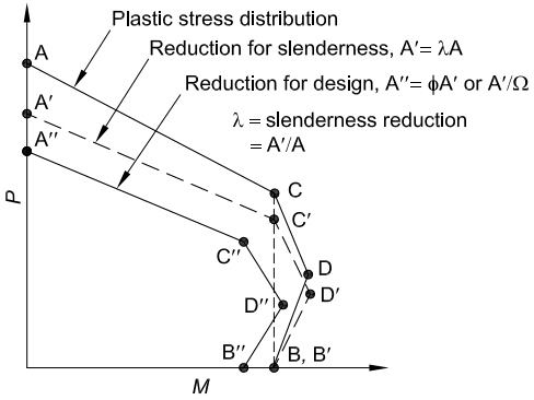
Figure description:
Interaction Diagram for Steel Sections Comparison of plastic stress distribution with slenderness and design reductions
P-M Interaction Curves
Legend
- Plastic stress distribution — color: black; symbol: Solid line
- Reduction for slenderness, A' = λ A — color: black; symbol: Dashed line
- Reduction for design, A'' = ϕ A' or A'/Ω — color: black; symbol: Solid line
Annotations
- λ = slenderness reduction = A'/A (text_label - position: top right region)
- Vertical alignment line connecting C, C', and B, B' (vertical_line - position: M = M_C = M_{C'} = M_B = M_{B'})
| Curve | Point (M=0) | Point (Intermediate 1) | Point (Intermediate 2) | Point (P=0) |
|---|---|---|---|---|
| Plastic stress distribution | A | C | D | B |
| Reduction for slenderness (A' = λ A) | A' | C' | D' | B' |
| Reduction for design (A'' = ϕ A' or A'/Ω) | A'' | C'' | D'' | B'' |
Notes: The chart illustrates three interaction curves for axial load (P versus moment (M. Points A, A', and A'' represent pure axial capacities (M=0. Points B, B', and B'' represent pure bending capacities (P=0. Points B and B' are coincident and vertically aligned with knee points C and C' on their respective curves. Points D, D', and D'' represent peak moment capacities.))))
Fig. C-I5.2. Interaction diagram for composite beam-columns—Method 2.
Specification for Structural Steel Buildings, August 1, 2022 AMERICAN INSTITUTE OF STEEL CONSTRUCTION
Using linear interpolation between points A", C", and B" in Figure C-I5.3, the following interaction equations may be derived for composite beam-columns subjected to combined axial compression plus biaxial flexure:
(a) If
(C-I5-1a)
(b) If
(C-I5-1b)
where For design according to Section B3.1 (LRFD):
required flexural strength using LRFD load combinations, kip-in. (N-mm)
- design flexural strength at point C", determined in accordance with Section I3, kip-in. (N-mm)
required compressive strength using LRFD load combinations, kips (N)
- = design axial compressive strength at point A" in Figure C-I5.3, determined in accordance with Section I2, kips (N)
design axial compressive strength at point C", kips (N)
For design according to Section B3.2 (ASD):
- required flexural strength using ASD load combinations, kip-in. (N-mm)
- required compressive strength using ASD load combinations, kips (N)
- = allowable compressive strength at point A" in Figure C-I5.3, determined in accordance with Section I2, kips (N)
allowable axial compressive strength at point C", kips (N)
- subscript relating symbol to major-axis bending
y
= subscript relating symbol to minor-axis bending
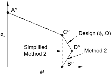
Figure description:
Comparison of Interaction Diagram Methods
M-P Interaction Diagram
Legend
- Method 2 — color: black; symbol: Solid line boundary A''-C''-D''-B''
- Simplified Method 2 — color: black; symbol: Dashed line segment C''-B''
Annotations
- Design (Δ, Β (text_label - position: Pointing to solid line segment C''-D''))
- Method 2 (text_label - position: Pointing to solid line segment D''-B'')
- Simplified Method 2 (text_label - position: Pointing to vertical dashed line segment C''-B'')
| Series / Path | Point 1 | M1 | P1 | Point 2 | M2 | P2 | Line Style |
|---|---|---|---|---|---|---|---|
| Method 2 / Design | A'' | 0 | 85 | C'' | 58 | 52 | Solid |
| Method 2 / Design | C'' | 58 | 52 | D'' | 70 | 28 | Solid |
| Method 2 / Design | D'' | 70 | 28 | B'' | 58 | 0 | Solid |
| Simplified Method 2 | A'' | 0 | 85 | C'' | 58 | 52 | Solid |
| Simplified Method 2 | C'' | 58 | 52 | B'' | 58 | 0 | Dashed |
Notes: The graph depicts an interaction diagram between axial load (P and bending moment (M. It compares Method 2, represented by a solid boundary passing through points A'', C'', D'', and B'', with Simplified Method 2, which utilizes a dashed vertical line connecting C'' to B'', effectively bypassing point D''. Points C'' and B'' share the same M-coordinate value.))
Fig. C-15.3. Interaction diagram for composite beam-columns—Method 2 simplified.
Method 3—Design Guide 6. The approach presented in AISC Design Guide 6 (Griffis, 1992) may also be used to determine the beam-column strength of encased W-shapes. Although this method is based on an earlier version of the Specification, available axial and flexural strengths can conservatively be determined directly from the tables in this design guide. The difference in resistance factors from the earlier Specification may safely be ignored.
Method 4—Direct Interaction Method for Noncompact Composite and Slender-Element Composite Filled Sections. For filled noncompact composite and slender-element composite members, the interaction equations in Section H1.1 can be conservative (Lai et al., 2016). The interaction between axial compression, , and flexure, , in filled composite members is typically seen to vary with the strength ratio, , which is calculated using Equation I5-2 as the yield strength of the steel components divided by the compressive strength of the concrete component. As the ratio increases, the steel component dominates. As the ratio decreases, the concrete component dominates.
This behavior is illustrated in Figure C-I5.4, which shows interaction curves developed using Equations I5-1a and b. Lai et al. (2016) developed these equations as a bilinear simplification of the parabolic interaction curves for filled composite members with noncompact composite or slender-element composite cross sections. The three anchor points of the normalized interaction curve include (a) the member available axial compressive strength as a column, , determined using Section I2.2b; (b) the member available flexural strength, , determined using Section I3.4;
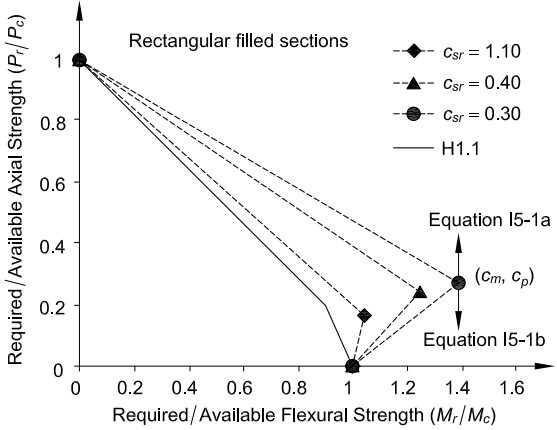
Figure description:
Rectangular Filled Sections Interaction Comparison Required / Available Axial Strength ( vs. Required / Available Flexural Strength (
Interaction Curves for Rectangular Filled Sections
Legend
- c_sr = 1.10 — color: black; symbol: Dashed line with diamond marker
- c_sr = 0.40 — color: black; symbol: Dashed line with triangle marker
- c_sr = 0.30 — color: black; symbol: Dashed line with circle marker
- H1.1 — color: black; symbol: Solid line
Annotations
- Rectangular filled sections (text_label - position: top center within plot)
- (c_m, c_p (text_label - position: y = 0.27, x = 1.4))
- Equation I5-1a (text_label - position: above (1.4, 0.27 with upward arrow))
- Equation I5-1b (text_label - position: below (1.4, 0.27 with downward arrow))
| Required / Available Flexural Strength () | Required / Available Axial Strength () for H1.1 | Required / Available Axial Strength () for | Required / Available Axial Strength () for | Required / Available Axial Strength () for |
|---|---|---|---|---|
| 0.0 | 1.0 | 1.0 | 1.0 | 1.0 |
| 0.9 | 0.2 | null | null | null |
| 1.0 | 0.0 | 0.0 | 0.0 | 0.0 |
| 1.05 | null | 0.17 | null | null |
| 1.25 | null | null | 0.24 | null |
| 1.4 | null | null | null | 0.27 |
Notes: The chart shows interaction curves comparing the AISC H1.1 standard curve with proposed equations (I5-1a and I5-1b for rectangular concrete-filled steel sections at various steel-to-concrete strength ratios (c_sr.))
Fig. C-15.4. Interaction diagram for filled composite members with noncompact composite or slender-element composite cross section developed using Equations 15-1a and b.
and (c) the balance point with coordinates . The balance point coordinates are functions of the strength ratio, , and calculated using Table I5.1 for rectangular and round filled composite members.
The interaction curve developed using Equations I5-1a and b is recommended for noncompact or slender-element filled composite members: (a) with governing unsupported length-to-diameter, , or length-to-width, , ratios less than or equal to 20; and (b) not providing stability support to gravity-only columns with significant axial loading. In situations where (a) and (b) are not met, the balance point with coordinates may be reduced further due to slenderness effects. This potential problem can be addressed through the simplified method described earlier and shown in Figure C-I5.3, where the increased available flexural strength due to axial compression is removed from the interaction curve.
The flexural capacity of composite plate shear walls subjected to axial compression can be estimated using the plastic stress distribution method of Section II.2a, or the effective stress-strain method of Section II.2d (Bruneau et al., 2019; Shafaei et al., 2021a, b). Bruneau et al. (2019) and Shafaei et al. (2021a) have reported the results of experimental investigations on planar walls subjected to different axial load and cyclic lateral loading up to failure.